Space-time dual cat and clock maps

Austen Lamacraft (Cambridge) and Pieter Claeys (Dresden)

austen.uk/#talks for slides

Motivation: kicked Ising model

• Time dependent Hamiltonian with kicks at $t=0,1,2,\ldots$

$$ \begin{aligned} H_{\text{KIM}}(t) = H_\text{I}[\mathbf{h}] + \sum_{m}\delta(t-n)H_\text{K}\\ H_\text{I}[\mathbf{h}]=\sum_{j=1}^L\left[J Z_j Z_{j+1} + h_j Z_j\right],\qquad H_\text{K} &= b\sum_{j=1}^L X_j \end{aligned} $$

• “Stroboscopic” form of $U(t)=\mathcal{T}\exp\left[-i\int^t H_{\text{KIM}}(t’) dt’\right]$

$$ \begin{aligned} U(n_+) &= \left[U(1_+)\right]^n,\qquad U(1_-) = K I_\mathbf{h}\\ I_\mathbf{h} &= e^{-iH_\text{I}[\mathbf{h}]}, \qquad K = e^{-iH_\text{K}} \end{aligned} $$

Unitary circuit

• Another class of discrete time dynamics

KIM as a circuit

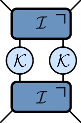
$$ \begin{aligned} \mathcal{K} &= \exp\left[-i b X\right]\\ \mathcal{I} &= \exp\left[-iJ Z_1 Z_2 -i \left(h_1 Z_1 + h_2 Z_2\right)/2\right] \end{aligned} $$

Expectation values

• Evaluate $\bra{\Psi}\mathcal{O}\ket{\Psi}=\bra{\Psi_0}\mathcal{U}^\dagger\mathcal{O}\mathcal{U}\ket{\Psi_0}$ for local $\mathcal{O}$

Folded picture

• After folding, lines correspond to two indices / 4 dimensions

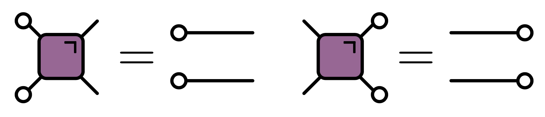
Unitarity in folded picture

• Circle denotes $\delta_{ab}$

$\bra{\Psi}\mathcal{O}\ket{\Psi}$ in folded picture

• Emergence of “light cone”

Reduced density matrix

• Expectation values in region $A$ evaluated using reduced density matrix

$$ \rho_A = \operatorname{tr}_{\bar A}\left[\ket{\Psi}\bra{\Psi}\right]=\operatorname{tr}_{\bar A}\left[\mathcal{U}\ket{\Psi_0}\bra{\Psi_0}\mathcal{U}^\dagger\right] $$

Toy model: SWAP circuit

• For a Bell pair consisting of qubits at sites $m$ and $n$:

  • If $n\in A$, $m\in\bar A$, $\rho_A$ has factor $\mathbb{1}_n$.

  • If $m, n\in A$ they contribute a factor $\ket{\Phi^+}_{nm}\bra{\Phi^+}_{nm}$ (pure)

• Only first case contributes to $ S_A = \min(4\lfloor t/2\rfloor, |A|) $ bits

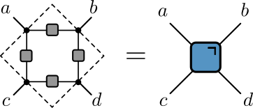
Dual unitary gates

• Impose additional restriction

• Gopalakrishnan and Lamacraft (2019), Bertini, Kos, and Prosen (2019)

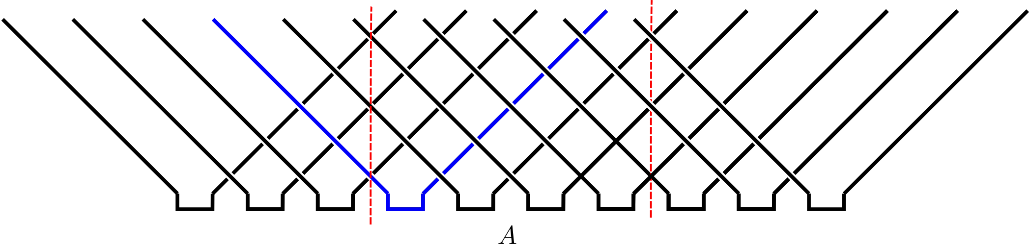
$\rho_A$ via dual unitarity

• 8 sites; 4 layers

• $\rho_A$ is unitary transformation of

$$ \mathbb{1}\otimes\mathbb{1}\otimes\mathbb{1}\otimes\mathbb{1}\otimes\mathbb{1}\otimes\mathbb{1}\otimes\mathbb{1}\otimes\mathbb{1} $$

Shallower…

• $\rho_A$ is unitary transformation of

$$ \mathbb{1}\otimes\mathbb{1}\ket{\Phi^+}\bra{\Phi^+}\otimes\ket{\Phi^+}\bra{\Phi^+}\otimes\mathbb{1}\otimes\mathbb{1} $$

General case

• RDM is unitary transformation of

$$ \rho_0=\overbrace{\frac{\mathbb{1}}{2}\otimes \frac{\mathbb{1}}{2} \cdots }^{t-1} \otimes\overbrace{\ket{\Phi^+}\bra{\Phi^+} \cdots }^{N_A/2-t+1 } \otimes \overbrace{\frac{\mathbb{1}}{2}\otimes \frac{\mathbb{1}}{2} \cdots }^{t-1} $$

• RDM has $2^{\min(2t-2,N_A)}$ non-zero eigenvalues all equal to $\left(\frac{1}{2}\right)^{\min(2t-2,N_A)}$

• Converse – maximal entanglement growth implies dual unitary gates – recently proved by Zhou and Harrow (2022)

Thermalization

• After $N_A/2 + 1$ steps, reduced density matrix is $\propto \mathbb{1}$

• All expectations (with $A$) take on infinite temperature value

The dual unitary family

• $4\times 4$ unitaries are 16-dimensional

• Family of dual unitaries is 14-dimensional

• Includes kicked Ising model at particular values of couplings

• Dual unitaries not “integrable” (except at special points) but have enough structure to allow many calculations

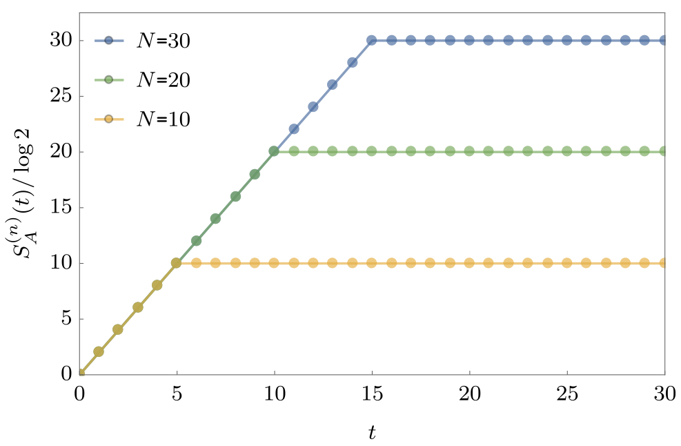
Entanglement Growth for Self-Dual KIM

• Bertini, Kos, Prosen (2019) found that when $|J|=|b|=\pi/4$

$$ \lim_{L\to\infty} S_A =\min(2t-2,N_A)\log 2, $$

• Any $h_j$; initial $Z_j$ product state

‘KIM’ property

• ($q=2$ here) Not satisfied by e.g. $\operatorname{SWAP}$

• Maps product states to maximally entangled (Bell) states

• Product initial states also work for KIM!

• Piroli et al (2020) studied more general initial states

Correlation functions

• Infinite temperature correlator $\tr\left[\sigma^\alpha_x(x,t)\sigma^\beta(y,0)\right]$

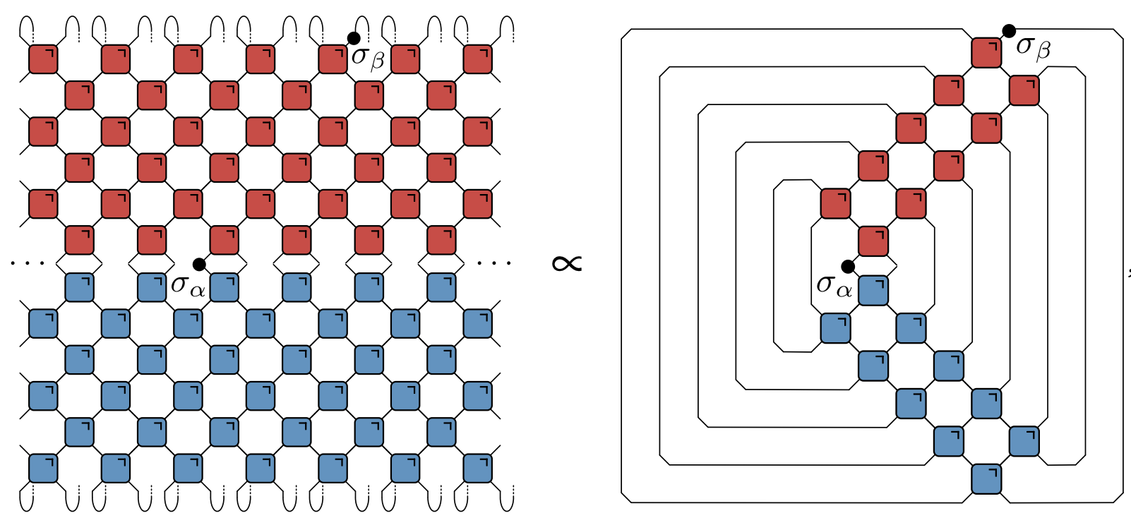
• Bertini, Kos, and Prosen (2019): dual unitarity means correlations vanish inside light cone!

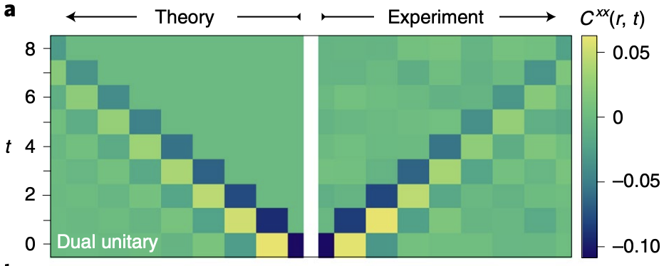
Quantinuum experiment

• Correlations measured in SDKIM last year

Outline

• Generalizing SDKI with Hadamard gates

• Cat maps and Clifford gates; classical limit

• Space-time duality for CA

• Models with continuous state space

• Recall KIM has circuit representation

$$ \begin{aligned} \mathcal{K} &= \exp\left[-i b X\right]\\ \mathcal{I} &= \exp\left[-iJ Z_1 Z_2 -i \left(h_1 Z_1 + h_2 Z_2\right)/2\right] \end{aligned} $$

• At $|J|=|b|=\pi/4$ model is dual unitary

“Seeing” dual unitarity

• At the dual unitary point $b=\pm i\pi/4$

$$ \mathcal{K} = \exp\left[\pm i \frac{\pi}{4} X\right]=\frac{1}{\sqrt{2}}\begin{pmatrix} 1 & \pm i \\ \pm i & 1 \end{pmatrix} $$

• Is $\propto$ Hadamard matrix: $|H_{ij}|=1$ with $H^\dagger H = d\mathbb{1}$

• Can be interpreted as diagonal phases when “viewed sideways”

• Back to lattice spin model picture

$$ U = \mathcal{N}\sum_{z_i\in \mathbb{Z}_d}\prod_{<i,j>} u_{ij}(z_i, z_j) $$

• $u_{ij}(z_i, z_j): \mathbb{Z}_d\times \mathbb{Z}_d\longrightarrow U(1)$

• $z_i=\omega_d^{n_i}$ for $n_i=0,\ldots d-1$, with $\omega_d = \exp(2\pi i/d)$

$$ U = \mathcal{N}\sum_{z_i\in \mathbb{Z}_d}\prod_{<i,j>} u_{ij}(z_i, z_j) $$

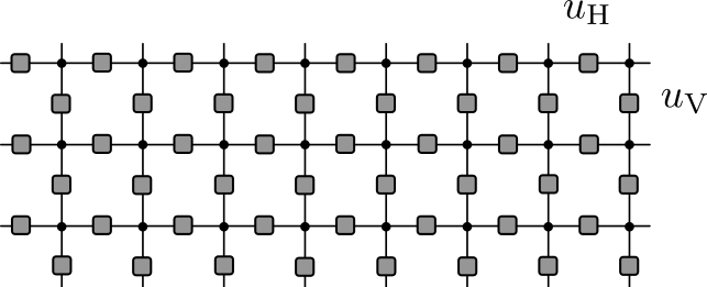
• When does this describe unitary evolution (vertically)?

• Single row $U_{\text{row }t}$ corresponds to diagonal operator

$$ \braket{z_{1:N,t}|U_{\text{row }t}|z_{1:N,t}} = \prod_{x=1}^N u_\text{H}(z_{x,t},z_{x+1,t}) $$

• Unitary since $u_\text{H}$ are phases

• Vertical bonds correspond to operators $u_\text{V}$ with matrix elements

$$ u_\text{V}(z_i,z_j)=\braket{z_i|u_\text{V}|z_j} $$

• Also unitary up to a multiplicative factor i.e. $u_\text{V}$ is Hadamard!

• In the same way, space-like evolution is unitary if $u_\text{H}$ is Hadamard

• If both $u_\text{V}$ and $u_\text{H}$ are Hadamard (e.g. SKDI): unitary evolution in both space and time or space-time duality (Gutkin et al. (2020))

Hadamard matrices

• Simple and important example is Fourier matrix (performs DFT)

$$ \left(F_d\right)_{jk} = \exp\left(2\pi ijk/d\right)\qquad j,k=0,\ldots, d-1 $$

• $H$ and $H'$ are equivalent if $$ H' = D_1P_1 H P_2 D_2 $$

• $D_{1,2}$ are diagonal unitaries and $P_{1,2}$ permutations

• If $D_1=D_2=\mathbb{1}$ $H$ and $H'$ are permutation equivalent

• Dephased form of a Hadamard matrix has first row and column all 1

• Two Hadamard matrices with same dephased form are equivalent

$$ \begin{align*} H_\text{deph} &= D_1 H D_2\\ D_1&= \operatorname{diag}(\bar H_{11},\bar H_{21},\ldots \bar H_{d1})\\ D_2&= \operatorname{diag}(1,H_{11}\bar H_{12},\ldots H_{11}\bar H_{1d}) \end{align*} $$

• $d=2,3$ and $5$: all complex Hadamard matrices equivalent to $F_d$ $$ F_2 = \begin{pmatrix} 1 & 1 \\ 1 & -1 \end{pmatrix} $$

• Equivalent to self-dual Ising kick matrix

$$ K_{2} =\begin{pmatrix} 1 & i \\ i & 1 \end{pmatrix}= \begin{pmatrix} 1 & 0\\ 0 & i \end{pmatrix} F_2\begin{pmatrix} 1 & 0\\ 0 & i \end{pmatrix} $$

• As a phase function

$$ K_{2}(z_i, z_j) = e^{i\pi/4}\exp\left(-\frac{i\pi}{4} z_i z_j\right) $$ $$ F_{2}(z_i, z_j) = e^{i\pi/4}\exp\left(\frac{i\pi}{4} \left[z_i z_j-z_i-z_j\right]\right) $$

• For $d=3$

$$ F_3 = \begin{pmatrix} 1 & 1 & 1 \\ 1 & \omega_3 & \omega_3^2 \\ 1 & \omega_3^2 & \omega_3 \end{pmatrix} $$

• Equivalent to

$$ K_3 = \begin{pmatrix} 1 & \omega_3 & \omega_3 \\ \omega_3 & 1 & \omega_3 \\ \omega_3 & \omega_3 & 1 \\ \end{pmatrix} $$

• Tensor product of Hadamards is Hadamard e.g.

$$ F_2\otimes F_2 = \begin{pmatrix} 1 & 1 & 1 & 1 \\ 1 & -1 & 1 & -1 \\ 1 & 1 & -1 & -1 \\ 1 & -1 & -1 & 1 \end{pmatrix} $$

• Permutation inequivalent to $F_4$. Full orbit of inequivalent Hadamards

$$ F_4^{(1)}(a)=\left[\begin{array}{cccc} 1 & 1 & 1 & 1 \\ 1 & i e^{i a} & -1 & -i e^{i a} \\ 1 & -1 & 1 & -1 \\ 1 & -i e^{i a} & -1 & i e^{i a} \end{array}\right]\qquad a \in [0,\pi) $$

• $F_4^{(1)}(0)=F_4$ and $F_4^{(1)}(\pm\pi/4)$ is perm equivalent to $F_2\otimes F_2$

Generalized Pauli matrices

$$ \begin{align*} Z_d = \begin{pmatrix} 1 & 0 & 0 & \cdots & 0\\ 0 & \omega_d & 0 & \cdots & 0\\ \cdots & \cdots & \cdots & \cdots & \cdots \\ 0 & 0 & 0 & \cdots & \omega_d^{d-1} \end{pmatrix}\\ X_d = \begin{pmatrix} 0 & 1 & 0 & \cdots & 0\\ 0 & 0 & 1 & \cdots & 0\\ \cdots & \cdots & \cdots & \cdots & \cdots \\ 1 & 0 & 0 & \cdots & 0 \end{pmatrix} \end{align*} $$

• Satsify $Z_d^d=X_d^d=\mathbb{1}$ and Weyl relation $X_d Z_d = \omega_d Z_d X_d$

• $Z^a X^b$ with $a,b=0,\ldots d-1$ form basis for local operators

• Quantum mechanical analogue of phase space torus $$ Z= e^{2\pi i q}\qquad X=e^{2\pi ip} $$

• Conjugating by Fourier matrix $$ F Z^a X^b F^\dagger = X^{a}Z^{-b} $$ like $-\pi/2$ rotation of torus: $(q,p)\longrightarrow (p,-q)$

Cat maps

$$ C_{jk}(\alpha,\delta)\equiv \exp\left(\frac{2\pi i}{d}\left[\frac{\alpha j^2}{2} + jk + \frac{\delta k^2}{2}\right]\right)\qquad \alpha,\delta\in \mathbb{Z} $$

• Area preserving (symplectic) linear map on torus $$ \begin{align*} \begin{pmatrix} q \\ p \end{pmatrix}&\longrightarrow \begin{pmatrix} q' \\ p' \end{pmatrix} = T \begin{pmatrix} q \\ p \end{pmatrix}\qquad \mod 1\nonumber\\ T &= \begin{pmatrix} \alpha & \beta \\ \gamma & \delta \end{pmatrix}\qquad \alpha,\beta,\gamma,\delta\in\mathbb{Z},\qquad \alpha\delta-\beta\gamma=1 \end{align*} $$

• $C_{jk}(\alpha,\delta)$ has $\beta=1$ and is Clifford: $Z^a X^b\longrightarrow Z^{a'} X^{b'}$

• Quantum cat maps first studied by Hannay and Berry (1980) as quantum analogs of classical Arnold cat maps

Arnold’s cat map

$$ T:\begin{pmatrix} q \\ p \end{pmatrix}\longrightarrow \begin{pmatrix} \alpha & 1 \\ \alpha\delta - 1 & \delta \end{pmatrix} \begin{pmatrix} q \\ p \end{pmatrix}\qquad \mod 1 $$

• Chaotic when one Lyapunov exponent exceeds one for $|\alpha+\delta|>2$.

$$ \begin{align*} T &= \begin{pmatrix} 2 & 1 \\ 3 & 2 \end{pmatrix}: C_{jk}(2,2) = \exp\left(\frac{2\pi i}{d}\left[j^2+k^2+jk\right]\right)\text{ (hyperbolic)}\nonumber\\ T &= \begin{pmatrix} -1 & 1 \\ 0 & -1 \end{pmatrix}: C_{jk}(-1,-1) = \exp\left(-\frac{i\pi}{d}\left[j-k\right]^2\right) \text{ (parabolic)} \end{align*} $$

• Second has $\mathbb{Z}_d$ clock symmetry: $j\longrightarrow j+1$ (mod $d$). Should become $U(1)$ symmetry in the $d\to\infty$ limit

• Parity of $d$ is important since $$ \exp\left(\frac{i\pi (j+d)^2}{d}\right)=(-1)^d \exp\left(\frac{i\pi j^2}{d}\right) $$

• Find update of general Pauli

$$ \prod_{x=1}^N Z^{a_{x,t}}X^{b_{x,t}}\qquad a_{x,t}, b_{x,t}\in \mathbb{Z}_d. $$

• Taking $u_\text{H}=F$ and $u_\text{V}=C(\alpha,\delta)$ (H then V)

$$ \begin{align*} a_{x,t+1} &= \alpha(a_{x,t}-b_{x-1,t}-b_{x+1,t}) + (\alpha\delta -1)b_{x,t}\nonumber\\ b_{x,t+1} &= a_{x,t} - b_{x-1,t} - b_{x+1,t}+\delta b_{x,t} \end{align*}\mod d $$

• `Hamiltonian’ form of equations of motion

• Second difference `Lagrangian’ formulation

$$ \begin{align*} \left[\Delta b\right]_{x,t} &= (\alpha + \delta - 4)b_{x,t}\qquad \mod d\nonumber\\ \left[\Delta b\right]_{x,t} &\equiv b_{x,t+1} + b_{x+1,t-1} + b_{x+1,t} + b_{x-1,t} - 4b_{x,t} \end{align*} $$

• Symmetry between space and time is evident

• Taking $u_\text{H}=F^\dagger$ and $u_\text{V}=C(\alpha,\delta)$

$$ \begin{align*} \left[\square b\right]_{x,t} &= (\alpha + \delta)b_{x,t}\qquad \mod d\nonumber\\ \left[\square b\right]_{x,t} &\equiv b_{x,t+1} + b_{x+1,t-1} - b_{x+1,t} - b_{x-1,t} \end{align*} $$

• For $\alpha=\delta=0$ particularly simple form

$$ \begin{align*} \left[\square b\right]_{x,t} &= 0 \end{align*} $$

• Left and right propagating solutions

$$ \begin{align*} a^R_{x,t} &= r_{x-t} \qquad b^R_{x,t} = -r_{x-t-1}\nonumber\\ a^L_{x,t} &= l_{x+t} \qquad b^L_{x,t} = -l_{x+t+1} \end{align*} $$

• General case: (Gütschow et al. (2010))

• Fourier transform of equation of motion

$$ M(u, u^{-1}) = \begin{pmatrix} \alpha & (\alpha\delta - 1) + \alpha(u + u^{-1}) \\ 1 & \delta + u + u^{-1} \end{pmatrix} $$

• $\operatorname{tr}M = \alpha + \delta + u + u^{-1}$ determines behaviour

• $\alpha+\delta=0$: glider automaton otherwise fractal

• Example: $d=3$, $u_\text{V}=C(1,0)$

• Local correlations vanish quickly!

Spatiotemporal cat

• Gutkin and Osipov (2016) define map on $N$ copies of torus

• Coupling between sites via $$ \begin{align*} x_{n}&\longrightarrow x_n \\ y_{n}&\longrightarrow y_n - x_{n-1} - x_{n+1} - V'(x_n) \end{align*}\qquad \mod 1 $$

• Generated by Hamiltonian (NB $V(x)$ periodic) $$ H_\text{c} = \sum_n \left[x_{n} x_{n+1} + V(x_n)\right] $$

• Alternate with cat maps $\mathcal{K}_n$ on each site

Lagrangian picture

• “Momenta” $y_n$ can be eliminated to give two-step (Lagrangian) recurrence for $x_{n,t}$: $$ [\Delta x]_{n,t} = (a+b-4)x_{n,t} - V'(x_{nt})-m_{n,t} \mod 1 $$ winding numbers $m_{n,t}$ chosen to ensure $x_{n,t}$ stays in the unit interval and $\Delta$ is the 2D Laplacian

Correlations

• Hu and Rosenhaus (2022), Fouxon and Gutkin (2022): explicit results for two and three site correlations.

• Correlations vanish for $t>\ell$, support of observable

• Christopoulos et al. (2023) and Lakshminarayan (2023) for correlations in other models

Lotkov et al. (2022)

• Floquet dynamics for $d=3$ $$ \begin{align*} H_1 &= \sum_{j=1}^{2N-1}\left(X_j^{\dagger}X_{j+1}+X_j X^{\dagger}_{j+1}\right)\\ H_2 &= \sum_{j=1}^{2N}\left(Z_j+Z_j^{\dagger}\right)\\ U_F &= e^{ifTH_2}e^{iJTH_1} \end{align*} $$

• Integrability conjectured for $fT = JT = \alpha_m$, with $\alpha_m = \frac{2\pi}{9}(2\ell-m)$, with $m=\pm 1$ and $\ell \in \mathbb{Z}$.

• Integrability subsequently established by Miao and Vernier (2023)

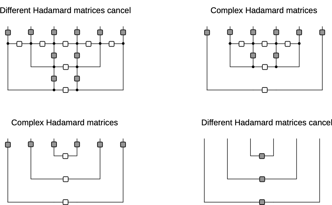
• Long range entanglement generation in integrable case

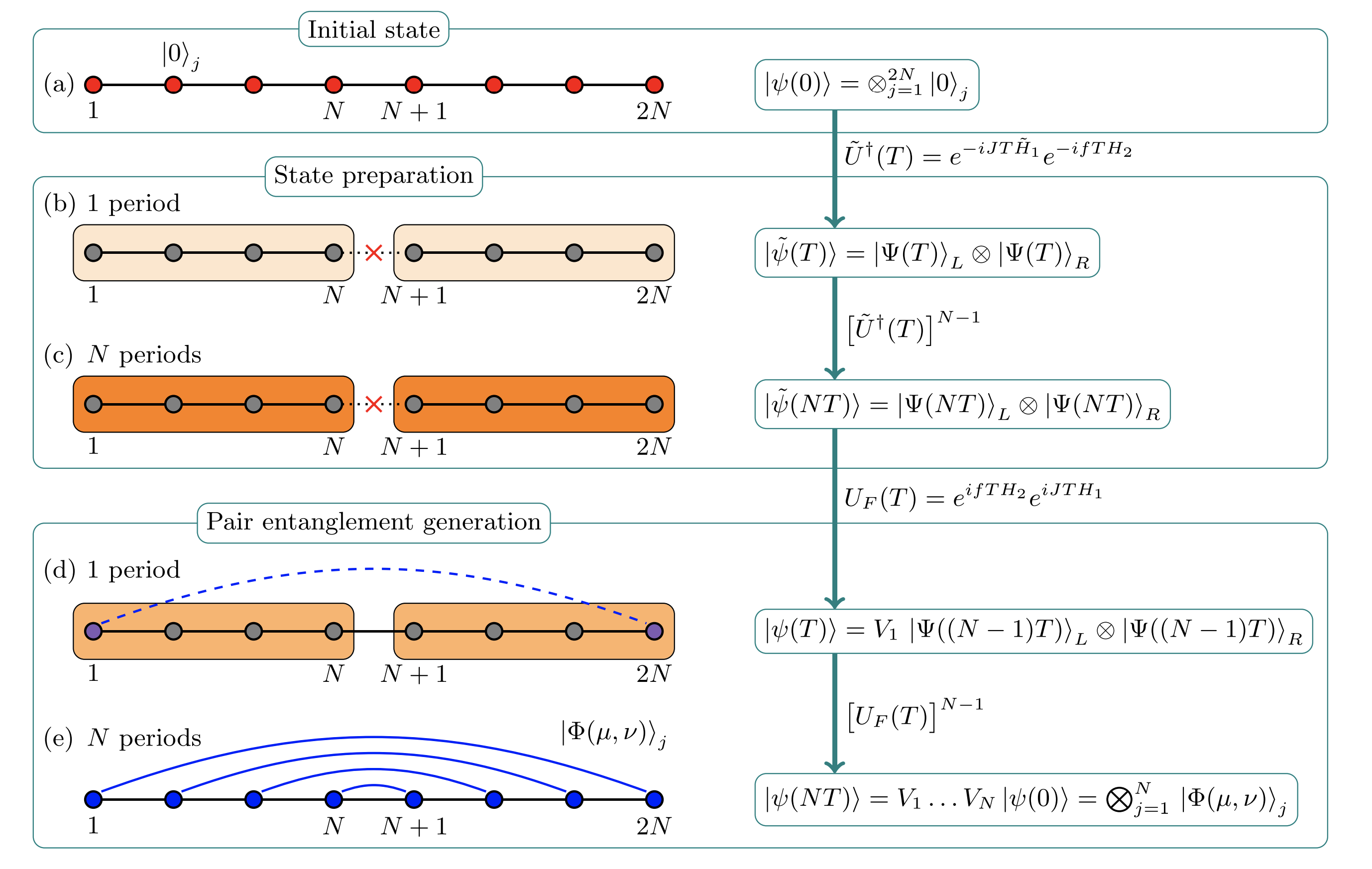
• Integrable case corresponds to

$$ \begin{align*} v_\text{H} = \begin{pmatrix} 1 & \omega & \omega \\ \omega & 1 & \omega \\ \omega & \omega & 1 \end{pmatrix} \qquad v_\text{V} = \begin{pmatrix} 1 & \omega^2 & \omega^2 \\ \omega^2 & 1 & \omega^2 \\ \omega^2 & \omega^2 & 1 \end{pmatrix}=\bar v_\text{H} \end{align*} $$

• $v_\text{H}$ dephases to $F$, so this is equivalent to $v_\text{H}=F$, $v_\text{V}=F^\dagger$

• Hence, ballistic propagation of operators

Diagrammatic derivation of rainbow state

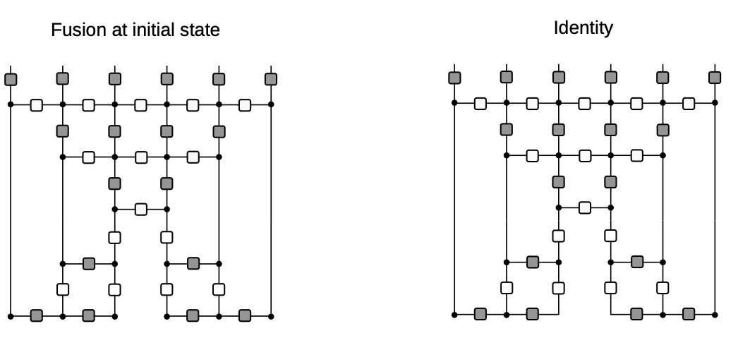
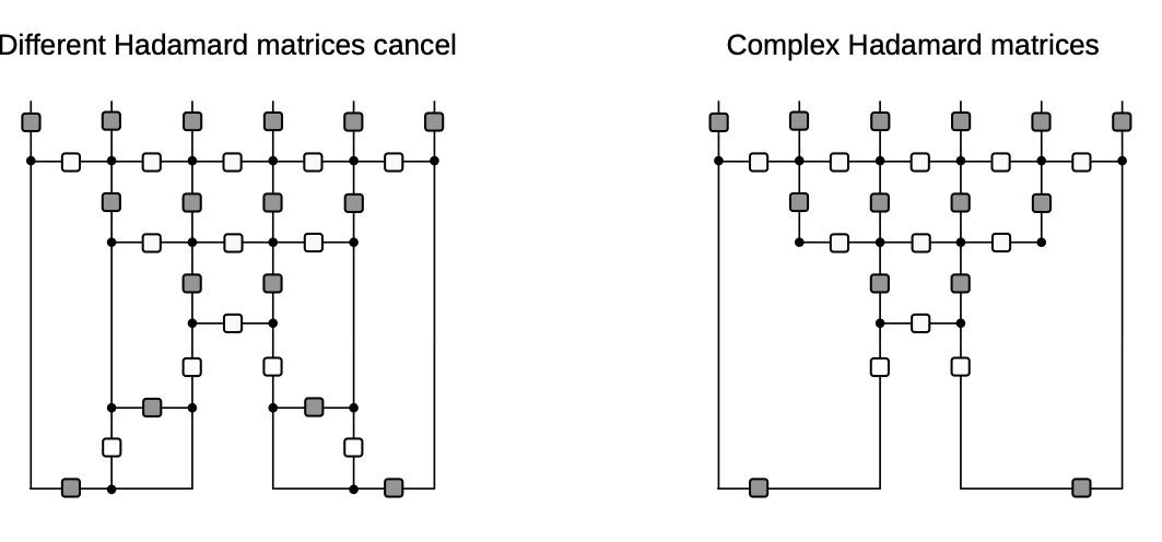
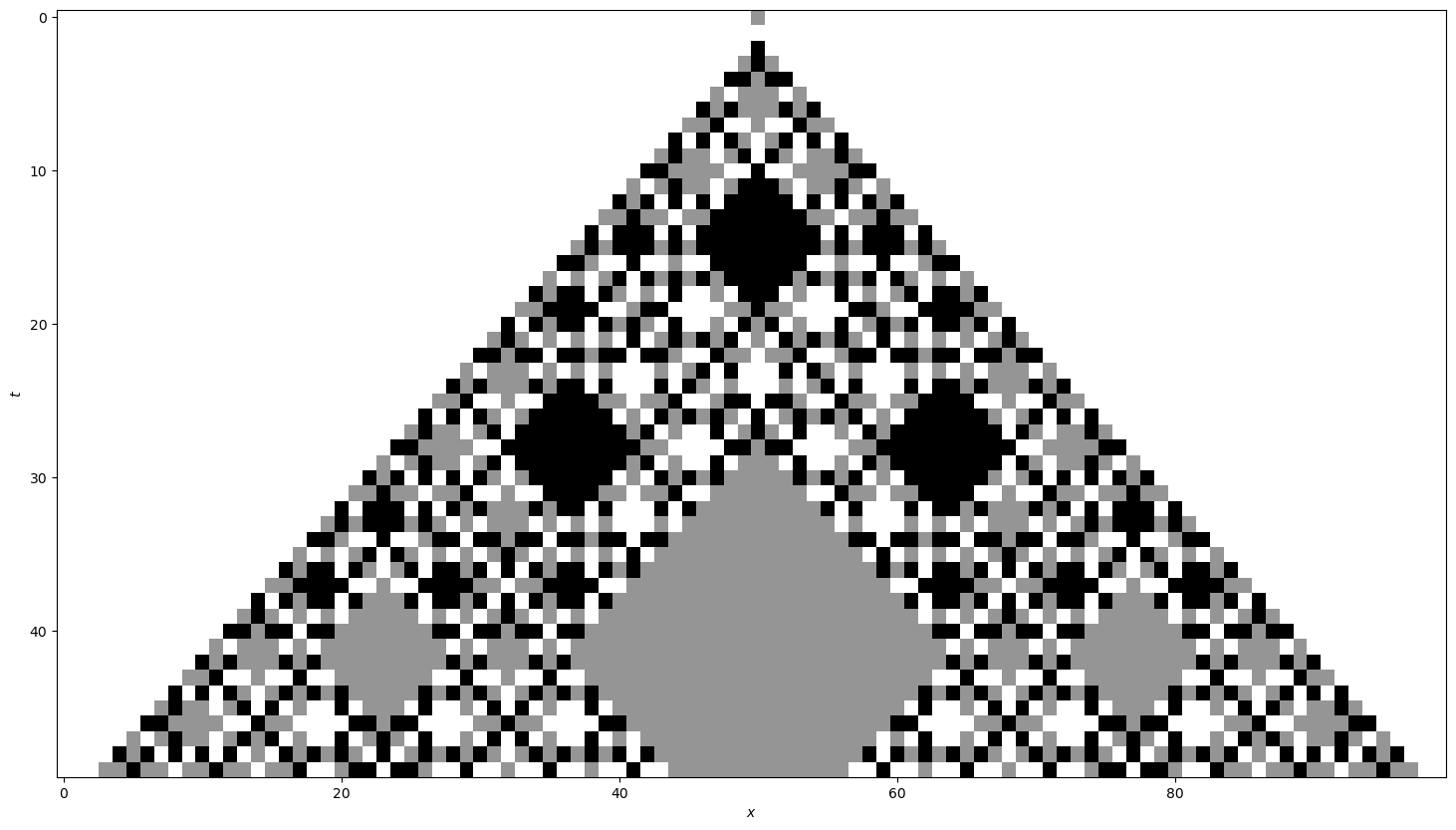
• Nonintegrable case

$$ v_\text{H} = v_\text{V} = \begin{pmatrix} 1 & \omega & \omega \\ \omega & 1 & \omega \\ \omega & \omega & 1 \end{pmatrix} $$

• Fractal operator dynamics

Questions

1. Do all integrable dual unitary circuits have “trivial” dynamics?

2. Is Fourier circuit model integrable in the usual sense (for $d>3$?)

3. Connect fractal behaviour of cats at finite $d$ to classical limit?

Dual unitarity for classical models?

Elementary cellular automata

• “Space” is one dimension with cells $x_n=0,1$ $n\in\mathbb{Z}$

• Update cells every time step depending on cells in neighborhood

• Neighborhood is cell and two neighbors for elementary CA

• Update specified by function

$$ f:\{0,1\}^3\longrightarrow \{0,1\}. $$

$$ x^{t+1}_{n} = f(x^{t}_{n-1},x^{t}_{n},x^{t}_{n+1}) $$

• How many possible functions?

Wolfram’s rules

• Domain of $f$ is $2^3=8$ possible values for three cells

• $2^8=256$ possible choices for the function $f$

• List outputs corresponding to inputs: 111, 110, … 000

• Interpret as binary number: this one is Rule 110

Elementary CA

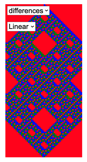
• Many behaviours, from ordered (Rule 18) to chaotic (Rule 30)

• Rule 110 is capable of universal computation!

CAs as model physics

• Notion of a causal “light cone” (45 degree lines)

• Variety of possible behaviours: chaos, periodicity, …

Chaos

• Rapid growth of small differences between two trajectories

• Smallest change: flip one site and monitor $z^t\equiv x^t\oplus y^t$

Chaos phenomenology

• No exponential growth (c.f. Lyapunov exponent in continuous systems)

• Track number of differences (Hamming distance) between trajectories

• Propagating “front” cannot exceed “speed of light”: generally slower

Reversibility

• No elementary CAs are reversible (bijective)!

• Reversibility is undecidable above one spatial dimension

• $∃$ reversible constructions

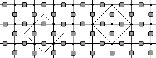
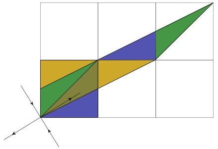
Block cellular automaton

• Partition cells into blocks (Margolus neighborhoods)
• Apply invertible mapping to block
• Alternate overlapping partitions

Spacetime representation

• Blue squares: invertible mapping on states of two sites: 00, 01, 10, 11

24 reversible models

• Each block a permutation of 00, 01, 10, 11

• $4!=24$ blocks

• Order:

  0. (0123)
  1. (0132)
  2. (0213), and so on

• Block 2 is the map $(00, 01, 10, 11) ⟶ (00, 10, 01, 11)$ (SWAP)

Reversible CA

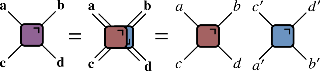
Circuit notation

$$ f:\Sigma\times\Sigma \longrightarrow\Sigma\times\Sigma, \qquad \Sigma=\{0,1\} $$

$$ (c,d) = f(a,b) $$

$$ F_{ab,cd} = \begin{cases} 1 & \text{if } (c,d) = f(a,b) \\ 0 & \text{otherwise} \end{cases} $$

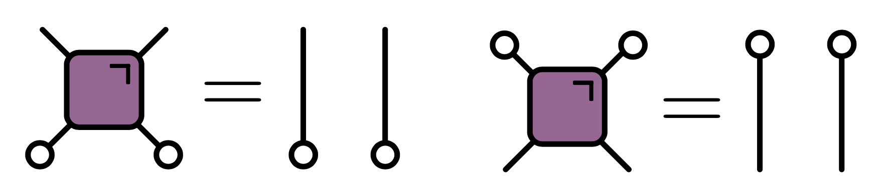
• If $f(\cdot,\cdot)$ is one-to-one:

$$ \sum_{a,b} F_{cd,ab} = \sum_{c,d} F_{cd,ab} = 1 $$

• Circle indicates sum over index

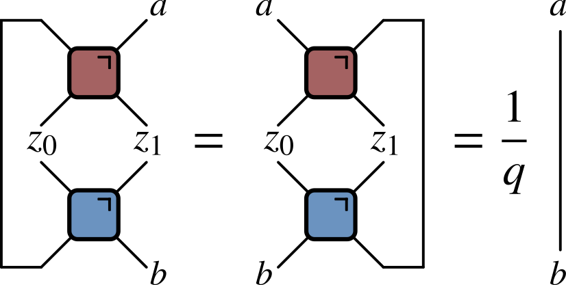
Dual reversibility

• If $(c,d)=f(a,b)$ require bijection $\tilde f$ satisfying $(d,b)=\tilde f(c,a)$

• In terms of $F_{ab,cd}$

$$ \sum_{a,c} F_{cd,ab} = \sum_{b,d} F_{cd,ab} = 1 $$

• Christopoulos et al. (2023), Lakshminarayan (2023)

Equivalent formulation

$$ \begin{align*} f(a,b)=(f_c(a,b),f_d(a,b))\\ \tilde f(c,a)=(\tilde f_d(c,a),\tilde f_b(c,a)) \end{align*} $$

• Dual reversibility implies that the maps $f_c(a,\cdot)$ and $f_d(\cdot,b)$ are bijections across diagonal

• “Nondegeneracy” in Etingof et al. (199), Gombor and Pozsgay (2022)

Three state models

• Of the 24 reversible blocks for two states, 12 are dual reversible

• Three states: Borsi and Pozsgay (2022) find 227 DR models

The linear block

$$ (c,d) = f(a,b) = (a + b, a - b), \mod 3 $$

• Original dual unitary circuit from Hosur et al.
• Unusual behaviour of recurrence time
  • For $L = 2\times 3^m$ have $T_\text{recur}=2L$
  • Borsi and Pozsgay prove using Fourier analysis over finite fields

Origin of “fractal” recurrence

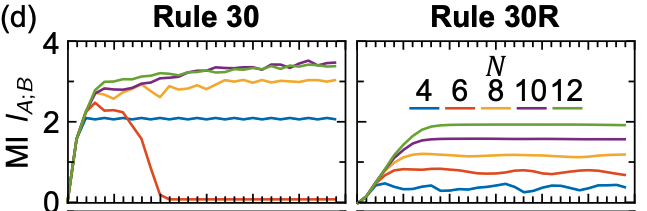
Mutual information

• Disjoint regions $A$ and $\bar A$: how much does one tell about the other?

• Use mutual information: measure of dependence of random variables

• Suggested in this context by Pizzi et al. (2022)

• MI defined as $$ I(X;Y) \equiv S(X) + S(Y) - S(X,Y) $$

  • $S(X)$ is entropy of $p_X(x)$; marginal distribution of $X$
  • $S(Y)$ is entropy of $p_Y(y)$; marginal distribution of $Y$
  • $S(X,Y)$ is entropy of joint distribution $p_{(X,Y)}(x,y)$

• Vanishes if $p_{(X,Y)}(x,y)=p_X(x)p_Y(y)$

Simple example

• Suppose either $X=Y=1$ or $X=Y=0$, with equal probability

$$ \begin{align*} p_{(X,Y)}(0,0)&=p_{(X,Y)}(1,1)=1/2\\ p_{(X,Y)}(1,0)&=p_{(X,Y)}(0,1)=0 \end{align*} $$

$$ I(X;Y)=S(X) + S(Y) - S(X,Y)= 1+1-1=1 \text{ bit} $$

Toy model (classical reprise)

• Initial distribution factorizes over correlated pairs
• Apply SWAPs
• 1 bit MI for every pair with one member in $A$ and one in $\bar A$

$$ I(A;\bar A) = \min(4\lfloor t/2\rfloor, |A|) \text{ bits} $$

• $|A|$ is (even) number of sites in $A$

Comments

• Total entropy conserved (c.f Liouville’s theorem)

• Entropy of initial distribution is half max, but entropy $S(A)$ saturates at maximal value (thermalization in time $\sim |A|/2$)

• This model is not so special! Any of the dual reversible BCAs behaves exactly the same!

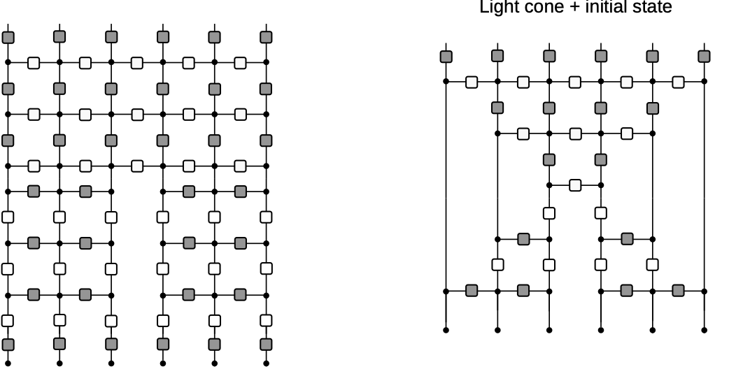
Graphical proof same as for dual unitaries

• $S(A)$ for 8 central sites
• Marginalize over $\bar A$

• After using dual reversibility, result is reversible automaton applied to initial state with $S(A)=6$ bits

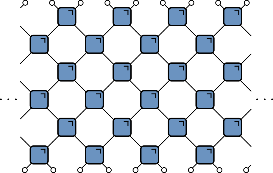
Models with continuous state space

$$ f:\Sigma\times\Sigma \longrightarrow\Sigma\times\Sigma $$

• Reversible: $f$ must be a bijection, so inverse $f^{-1}$ exists

• Probability distribution $p(a,b)$ on two sites is mapped to a distribution $$ p_f(c,d) = |\det Df|^{-1} p(f^{-1}(c,d)), $$ $Df$ is Jacobian matrix

• Impose $|Df|=1$: preserve uniform distribution

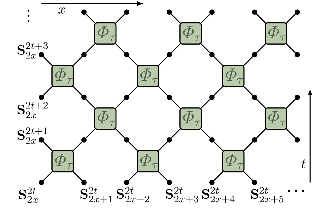
Krajnik-Prosen model

• Classical circuit, Symplectic map on $S^2\times S^2$

$$ \begin{align*} \Phi_{\tau}\left(\mathbf{S}_{1}, \mathbf{S}_{2}\right) &=\frac{1}{\sigma^{2}+\tau^{2}}\left(\sigma^{2} \mathbf{S}_{1}+\tau^{2} \mathbf{S}_{2}+\tau \mathbf{S}_{1} \times \mathbf{S}_{2}, \sigma^{2} \mathbf{S}_{2}+\tau^{2} \mathbf{S}_{1}+\tau \mathbf{S}_{2} \times \mathbf{S}_{1}\right) \\ \mathbf{S}_1^2&=\mathbf{S}_1^2=1\qquad \sigma^{2} =\frac{1}{2}\left(1+\mathbf{S}_{1} \cdot \mathbf{S}_{2}\right) \end{align*} $$

“Space-time duality” of KP model

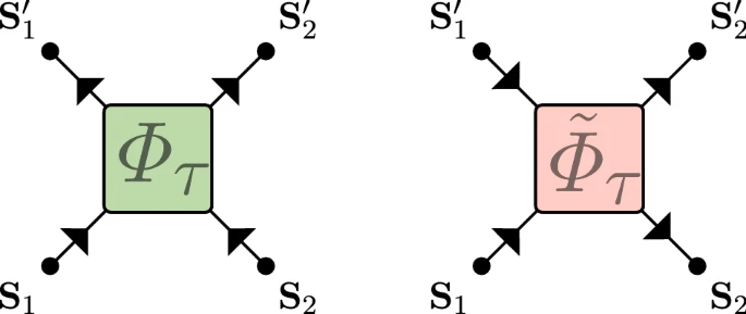
• $\tilde\Phi_\tau$ coincides with $\Phi_\tau$ after flipping

$$ \mathbf{S}_x^t \longrightarrow \tilde{\mathbf{S}}_x^t = (-1)^{x+t+1}\mathbf{S}_x^t $$

Nonzero correlations in the KP model

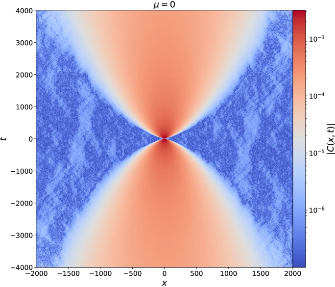
Model is not space-time dual in same sense as dual unitary circuits!

Dual reversibility

• As before $(d,b) = \tilde f(c,a)$. Require $|D \tilde f|=1$

• Discrete case: bijectivity of $\tilde f$ equivalent to existence of diagonal bijections $f_c(a,\cdot):\Sigma_b\longrightarrow \Sigma_c$ and $f_d(\cdot,b):\Sigma_a\longrightarrow \Sigma_d$

• Continuous case: additionally, bijections have unit determinant

• Recall $$ p_f(c,d) = |\det Df|^{-1} p(f^{-1}(c,d)) $$
• Equivalent to $$ p_f(c,d) = \int \delta((c,d)-f(a,b)) p(a,b)\, d\mu(a) d\mu(b) $$ $$ 1 = \int \delta((c,d)-f(a,b))\, d\mu(a) d\mu(b) $$

• $|D\tilde f|=1$ guarantees that

$$ 1 = \int \delta((d,b)-\tilde f(c,a))\, d\mu(a) d\mu(c) $$

• Not analog of

• Even if $(c,d)=f(a,b)$ and $(d,b)=\tilde f(c,a)$: $$ \delta((c,d)-f(a,b))\neq \delta((d,b)-\tilde f(c,a)) $$

Necessary condition

$$ \delta((c,d)-f(a,b))= \delta((d,b)-\tilde f(c,a)) $$

• Requires diagonal bijections satisfy

$$ |Df_c(a,\cdot)|=1\qquad |Df_d(\cdot,b)|=1 $$

• Not satisfied by Krajnik—Prosen model!

Symplectic dynamics

• State space $\Sigma$ is symplectic manifold with symplectic form $\omega$

• $f:\Sigma\times\Sigma\longrightarrow\Sigma\times\Sigma$ obeys $f^{*}(\omega_1+\omega_2)=\omega_1+\omega_2$

• $\omega$ has (locally) canonical form

$$ \omega = \sum_{i=1}^{n} dx_i\wedge dy_i $$

• $Df$ is symplectic matrix

$$ \begin{align*} Df^T \Omega Df &= \Omega\qquad \Omega \equiv\operatorname{diag}(\omega,\omega)\\ \omega &= \begin{pmatrix} 0 & \mathbb{1}_n \\ -\mathbb{1}_n & 0 \end{pmatrix} \end{align*} $$

• Rearranging gives condition on spatial Jacobian $D\tilde f$ $$ D\tilde f^T\operatorname{diag}(\omega,-\omega) D\tilde f = \operatorname{diag}(-\omega,\omega). $$

• $\tilde f$ not symplectic but may be made so by composing with pair of maps $\tau_{1,2}$ that reverse signs of $\omega_1$ and $\omega_2$ e.g. $\tau_{1,2}$ $y_i\to -y_i$

• $\tau_2\circ \tilde f\circ \tau_1$ is then symplectic

• In Krajnik—Prosen model this corresponds to $$ \mathbf{S}_x^t \longrightarrow \tilde{\mathbf{S}}_x^t = (-1)^{x+t+1}\mathbf{S}_x^t $$

• Any symplectic map volume preserving in spatial direction

Summary

• There is a “useful” notion of space-time duality for classical models

• Existing examples: spatiotemporal cat, dual unitary Cliffords

• New examples: Christopoulos et al. (2023) (classical spins) and Lakshminarayan (2023) (coupled standard maps)

Thank you!