\[ \nonumber \newcommand{\cE}{\mathcal{E}} \newcommand{\cH}{\mathcal{H}} \newcommand{\cN}{\mathcal{N}} \newcommand{\cC}{\mathcal{C}} \newcommand{\br}{\mathbf{r}} \newcommand{\bp}{\mathbf{p}} \newcommand{\bk}{\mathbf{k}} \newcommand{\bq}{\mathbf{q}} \newcommand{\bv}{\mathbf{v}} \newcommand{\pop}{\psi^{\vphantom{\dagger}}} \newcommand{\pdop}{\psi^\dagger} \newcommand{\Pop}{\Psi^{\vphantom{\dagger}}} \newcommand{\Pdop}{\Psi^\dagger} \newcommand{\Phop}{\Phi^{\vphantom{\dagger}}} \newcommand{\Phdop}{\Phi^\dagger} \newcommand{\phop}{\phi^{\vphantom{\dagger}}} \newcommand{\phdop}{\phi^\dagger} \newcommand{\aop}{a^{\vphantom{\dagger}}} \newcommand{\adop}{a^\dagger} \newcommand{\bop}{b^{\vphantom{\dagger}}} \newcommand{\bdop}{b^\dagger} \newcommand{\cop}{c^{\vphantom{\dagger}}} \newcommand{\cdop}{c^\dagger} \newcommand{\Nop}{\mathsf{N}^{\vphantom{\dagger}}} \newcommand{\bra}[1]{\langle{#1}\rvert} \newcommand{\ket}[1]{\lvert{#1}\rangle} \newcommand{\inner}[2]{\langle{#1}\rvert #2 \rangle} \newcommand{\braket}[3]{\langle{#1}\rvert #2 \lvert #3 \rangle} \DeclareMathOperator{\sgn}{sgn} \DeclareMathOperator{\tr}{tr} \newcommand{\abs}[1]{\lvert{#1}\rvert} \newcommand{\brN}{\br_1, \ldots, \br_N} \newcommand{\xN}{x_1, \ldots, x_N} \newcommand{\zN}{z_1, \ldots, z_N} \]
There are many situations in which an approach based on finite orders of perturbation theory either misses important physics, or leads to divergences (often both). In this lecture we develop many body perturbation theory in more detail by considering a formalism to calculate the partition function or free energy. We apply this approach to a toy model for electrons in a metal: a gas of fermions interacting via the Coulomb force in a neutralizing background of uniform charge density that plays the role of the ionic lattice. This is Jellium.
Dimensionless parameters
The Jellium Hamiltonian describing fermions interacting via the Coulomb interaction is (we ignore spin)
\[ H = \int \frac{1}{2m}\nabla\pdop\cdot\nabla\pop + \overbrace{\frac{1}{2}\int d\br d\br' :\left[\rho(\br)-n \right]U(\br-\br')\left[\rho(\br')-n\right]:}^{\equiv H_\text{int}}. \label{jelliumH} \]
Here, as usual, \(\rho(\br)=\pdop(\br)\pop(\br)\) is the number density operator, \(:(\cdots):\) denotes normal ordering, and \(\rho(\br)-n\) is the deviation from the uniform background charge. The two body interaction is
\[ U(\br) = \frac{e^2}{\abs{\br}} \]
(in Electrostatic units). A basic question is: what is the relative magnitude of the kinetic and potential terms? For a free fermion gas in its ground state, the kinetic energy per particle is \(\frac{3}{5}E_F\). Since \(n = \frac{k_\text{F}^3}{6\pi^2}\) this scales with density as \(n^{2/3}\). The scaling of the interaction energy is \(n^{1/3}\), showing that (perhaps counterintuitively) low density corresponds to strong interactions, relatively speaking. An appropriate dimensionless parameter is the ratio of the Wigner–Seitz radius to the Bohr radius \(r_\text{Bohr} = (me^2)^{-1}\) for our system. This gives
\[ \frac{r_s}{r_\text{Bohr}} = \left(\frac{3}{4\pi n}\right)^{1/3} me^2. \]
We have already encountered the following states in Fermi gases, roughly in order of increasing interaction strength:
The Landau Fermi liquid.
Ferromagnetism, when the Stoner criterion is reached. Although we discussed a microscopic calculation, the same criterion can easily be phrased in terms of the Landau function \(G(\phi)\).
Mott states that can occur in a lattice potential, giving insulating behaviour in systems band theory predicts to be metallic.
For very strong interactions, corresponding \(r_s\) values greater than 100, the system can form a Wigner crystal, breaking the continuous symmetry of spatial translations.
Using perturbation theory to go beyond the Hartree–Fock approximation leads to divergences in the case of Coulomb interactions. As a result, certain contributions to the perturbation series have to be summed to all orders. Far from being a mere technical nuisance, this resummation is linked to real physical effects arising from the long-ranged interaction, namely screening and collective excitations corresponding to quantized plasma oscillations.
Perturbation Series for the Partition Function
We are going to begin in very general terms, and consider the calculation of the (grand canonical) partition function
\[ Z = \tr\left[\exp\left(-\beta H\right)\right], \]
where \(H=H_0+H_\text{int}\), and \(H_0\) is the free particle Hamiltonian including the chemical potential, which we can write
\[ H_0 = \sum_\bk \xi(\bk)\adop_\bk \aop_\bk, \]
where \(\xi(\bk)=\epsilon(\bk)-\mu\). All thermodynamic quantities can be obtained from \(Z\), and the formalism can be further extended to calculate correlation functions.
The key to our approach is to exploit then analogy between the ‘Boltzmann operator’ \(e^{-\beta H}\) and the unitary time evolution operator \(U(t) = e^{-iHt}\). Calculating the partition function seems to involve evolution for imaginary time \(-i\beta\)! This suggests we can develop an interaction picture, just as in the real time case. We have the equation of motion
\[ \frac{d}{d\tau}\exp(-\tau H) = -\left(H_0+H_\text{int}\right)\exp(-\tau H). \]
Multiplying on the left by \(e^{\tau H_0}\) gives an equation satisfied by \(e^{\tau H_0}e^{-\tau H}\)
\[ \frac{d}{d\tau}\left[e^{\tau H_0}e^{-\tau H}\right] = -H_\text{int}(\tau)\left[e^{\tau H_0}e^{-\tau H}\right], \label{int_pic} \]
where \(H_\text{int}(\tau)\equiv e^{\tau H_0} H_\text{int}e^{-\tau H_0}\) corresponds to the perturbation in the interaction picture at time \(t=-i\tau\). The formal solution to \(\eqref{int_pic}\) at \(\tau=\beta\)
\[ e^{\beta H_0}e^{-\beta H} = T_\tau \exp\left(-\int_0^\beta H_\text{int}(\tau)d\tau\right), \]
where \(T_\tau\) is the operation of time ordering of the exponent, which is a shorthand for
\[ \begin{align} &T_\tau \exp\left(-\int_0^\beta H_\text{int}(\tau)d\tau\right) = 1 - \int_0^\beta H_\text{int}(\tau_1)d\tau_1\nonumber \\ \qquad &+ \int_0^\beta d\tau_2 \int_0^{\tau_2} d\tau_1 H_\text{int}(\tau_2)H_\text{int}(\tau_1)\nonumber \\ &\qquad- \int_0^\beta d\tau_3 \int_0^{\tau_3} d\tau_2 \int_0^{\tau_2} d\tau_1 H_\text{int}(\tau_3)H_\text{int}(\tau_2)H_\text{int}(\tau_1)+\cdots, \end{align} \]
with the times increasing from right to left. This gives our final expression for the partition function
\[ Z = \tr\left[e^{-\beta H_0}T_\tau \exp\left(-\int_0^\beta H_\text{int}(\tau)d\tau\right)\right]. \]
Perturbation theory then involves computing averages of a string of \(H_\text{int}(\tau)\) operators with respect to the Boltzmann distribution of the free Hamiltonian.
Wick’s Theorem
Let’s see how this works by considering the lowest order term when \(H_\text{int}\) is given by \(\eqref{jelliumH}\). In this case we just have to compute the thermal average of \(H_\text{int}\): the time dependence vanishes by virtue of the cyclic property of the trace. Writing out the perturbation in terms of the Fourier modes gives
\[ H_\text{int} = \frac{1}{2V} \sum_{\bk_1+\bk_2=\bk_3+\bk_4} U_{\bk_1-\bk_4} :(\adop_{\bk_1}\aop_{\bk_4}-nV\delta_{\bk_1,\bk_4})(\adop_{\bk_2}\aop_{\bk_3}-nV\delta_{\bk_2,\bk_3}):, \label{Hint_exp} \]
where
\[ U_\bq = \frac{4\pi e^2}{\abs{\bq}^2} \]
is the Fourier transform of the Coulomb potential. We have already discussed the expectation value of \(H_\text{int}\) in a product state in Lecture 6. Recall that the Hartree and Fock terms arise from two different ‘pairings’ of creation operators with annihilation operators. This sum over different pairings is a feature of expectations in a product state. Since \(e^{-\beta H_0}\) represents a statistical mixture of product states in which the occupation of each momentum state is independent
\[ e^{-\beta H_0} =\prod_\bk e^{-\beta\xi(\bk)N_\bk}, \]
we just set \(N_\bk\to \langle N_\bk\rangle\) in our earlier expression. We are now denoting the quantum and thermal expectation by single angular brackets to avoid clutter. Thus, for some operator \(A\)
\[ \langle A\rangle \equiv \frac{\tr\left[e^{-\beta H_0} A\right]}{Z_0},\quad Z_0 = \tr e^{-\beta H_0} \]
The importance of including the background charge density now becomes clear: the Hartree term vanishes (without the background charge it would be infinite!), leaving only the Fock term
\[ \langle H_\text{int}\rangle = - \frac{1}{2V} \sum_{\bk_1,\bk_2} U_{\bk_1-\bk_2} \langle N_{\bk_1}\rangle\langle N_{\bk_2}\rangle. \]
Before considering a situation where the time dependence enters in an essential way, let’s look at a slightly more general example of an expectation value
\[ \begin{align} \langle \pdop(\br_1)\pop(\br_2)\pdop(\br_3)\pop(\br_4)\rangle &= \frac{1}{V^2}\sum_{\bk_1,\bk_2,\bk_3,\bk_4} e^{i(-\bk_1\cdot\br_1+\bk_2\cdot\br_2-\bk_3\cdot\br_3+\bk_4\cdot\br_4)} \langle \adop_{\bk_1}\aop_{\bk_2}\adop_{\bk_3}\aop_{\bk_4} \rangle\nonumber\\ &= \frac{1}{V^2}\sum_{\bk_1,\bk_3} e^{i[\bk_1\cdot(\br_2-\br_1)+\bk_3\cdot(\br_4-\br_3)]} \langle \adop_{\bk_1}\aop_{\bk_1}\rangle\langle\adop_{\bk_3}\aop_{\bk_3} \rangle\nonumber\\ &\quad+ \frac{1}{V^2}\sum_{\bk_1,\bk_2} e^{i[\bk_1\cdot(\br_4-\br_1)+\bk_2\cdot(\br_2-\br_3)]} \langle \adop_{\bk_1}\aop_{\bk_1}\rangle\langle\adop_{\bk_2}\aop_{\bk_2} \rangle +\cdots\nonumber\\ &=\langle \pdop(\br_1)\pop(\br_2)\rangle\langle\pdop(\br_3)\pop(\br_4)\rangle \nonumber\\ &\quad+\langle \pdop(\br_1)\pop(\br_4)\rangle\langle\pop(\br_2)\pdop(\br_3)\rangle . \label{Wick_Example} \end{align} \]
The dots in the second equality are the accounting errors that we argued in Lecture 6 can be ignored in the thermodynamic limit. There are no signs on account of the even number of transpositions to shift things into order in the second term. On the other hand
\[ \begin{align} \langle \pdop(\br_1)\pdop(\br_2)\pop(\br_3)\pop(\br_4)\rangle =\langle \pdop(\br_1)\pop(\br_4)\rangle\langle\pdop(\br_2)\pop(\br_3)\rangle\nonumber\\ \quad\pm\langle \pdop(\br_1)\pop(\br_3)\rangle\langle\pdop(\br_2)\pop(\br_4)\rangle, \end{align} \]
with the plus sign for bosons and the minus sign for fermions. Hopefully the picture is clear: we sum over all possible pairings of creation with annihilation operators. For fermions we must in addition be careful to include a minus sign when, in moving paired creation and annihilation operators into position next to each other, we perform an odd number of transpositions.
The second order contribution to the partition function depends on
\[ \langle T_\tau H_\text{int}(\tau_2)H_\text{int}(\tau_1)\rangle. \label{2nd_Hint} \]
This is a function of \(\tau_1-\tau_2\), again as a result of the cyclic property. Including the time dependence in \(\eqref{Hint_exp}\) is straightforward
\[ H_\text{int}(\tau) = \frac{1}{2V} \sum_{\bk_1+\bk_2=\bk_3+\bk_4} U_{\bk_1-\bk_4} :(\adop_{\bk_1}(\tau)\aop_{\bk_4}(\tau)-nV)(\adop_{\bk_2}(\tau)\aop_{\bk_3}(\tau)-nV):, \label{Hint_exp_TD} \]
where the time dependence of the Fourier components is
\[ \aop_\bk(\tau) = e^{-\tau\xi(\bk)}\aop_\bk,\quad \adop_\bk(\tau) = e^{\tau\xi(\bk)}\adop_\bk. \]
How to we evaluate expectations of time ordered products? It’s fairly clear that our example \(\eqref{Wick_Example}\) is also an identity in this case
\[ \begin{align} &\langle T_\tau\pdop(\br_1,\tau_1)\pop(\br_2,\tau_2)\pdop(\br_3,\tau_3)\pop(\br_4,\tau_4)\rangle=\nonumber\\ &\qquad\langle T_\tau\pdop(\br_1,\tau_1)\pop(\br_2,\tau_2)\rangle\langle T_\tau\pdop(\br_3,\tau_3)\pop(\br_4,\tau_4)\rangle\nonumber\\ &\qquad\qquad+\langle T_\tau\pdop(\br_1,\tau_1)\pop(\br_4,\tau_4)\rangle\langle T_\tau\pop(\br_2,\tau_2)\pdop(\br_3,\tau_3)\rangle, \label{Wick_ExampleT} \end{align} \]
because the operators appear in the right time order in the expectation values on both sides. In turns out that this works for fermions too, provided that we define time ordering to include a sign corresponding to the signature of the permutation involved in putting the operators in time order. In the simplest case:
\[ \langle T_\tau \pdop(\br,\tau)\pop(\br',\tau') \rangle = \begin{cases} \langle \pdop(\br,\tau)\pop(\br',\tau') \rangle & \tau>\tau'\\ -\langle \pop(\br',\tau')\pdop(\br,\tau) \rangle & \tau'>\tau.\ \label{Fermi_Tdef} \end{cases} \]
To see why this is necessary, consider the expectation corresponding to the time ordering \(\tau_1>\tau_3>\tau_2>\tau_4\)
\[ \begin{align} &\langle\pdop(\br_1,\tau_1)\pdop(\br_3,\tau_3)\pop(\br_2,\tau_2)\pop(\br_4,\tau_4)\rangle=\nonumber\\ &\qquad-\langle \pdop(\br_1,\tau_1)\pop(\br_2,\tau_2)\rangle\langle \pdop(\br_3,\tau_3)\pop(\br_4,\tau_4)\rangle\nonumber\\ &\qquad\qquad+\langle \pdop(\br_1,\tau_1)\pop(\br_4,\tau_4)\rangle\langle \pdop(\br_3,\tau_3)\pop(\br_2,\tau_2)\rangle. \end{align} \]
Since the first term on the right hand side contains time ordered products, this identity is only described correctly by \(\eqref{Wick_ExampleT}\) if we use the above convention.
One further note about \(T_\tau\)-products: operators appearing in a \(T_\tau\) product can be regarded as (anti-)commuting, because the actual order that they appear in depends on their \(\tau\) labels. For instance \(T_\tau A(\tau_1)B(\tau_2) = \pm T_\tau B(\tau_2)A(\tau_1)\), depending on whether the operators are bosonic or fermionic.
To outcome of this discussion is Wick’s theorem:
An expectation of a \(T_\tau\)-product of operators with respect to a free Hamiltonian can be written as a sum of terms corresponding to all possible pairings of the operators. Each term consists of the product of \(T_\tau\)-product expectations for each pair. In the case of fermions, each term will have a sign corresponding to the signature of the permutation reordering the operators so that paired operators are adjacent.
This is the basic result used for evaluating the time ordered products like \(\eqref{2nd_Hint}\).
Green’s functions
In light of Wick’s theorem, we see that the basic quantity that appears in perturbation theory is
\[ G(\br,\tau,\br',\tau')\equiv\langle T_\tau \pop(\br,\tau)\pdop(\br',\tau') \rangle. \label{GF_def} \]
This is called a Green’s function, because it satisfies the equation
\[ \left[\partial_\tau + H_0\right]G(\br,\tau,\br',\tau')=\delta(\tau-\tau')\delta(\br-\br'). \label{GF_eq} \]
Make sure you understand where those \(\delta\)-functions on the right hand side come from!
The name is slightly unfortunate, because \(G(\br,\tau,\br',\tau')\) has a physical meaning in its own right, apart from being useful in perturbation calculation, and we can define it for an interacting system by taking expectations in \(\eqref{GF_def}\) with respect to the density matrix of the interacting system. In that case, however, \(G(\br,\tau,\br',\tau')\) does not obey a differential equation like \(\eqref{GF_eq}\). So in general many body Green’s functions are not Green’s functions in the sense of differential equations. Just to confuse you.
For the noninteracting Green’s functions that appear in our perturbation calculations \(\eqref{GF_eq}\) is very useful, allowing us to find \(G(\br,\tau,\br',\tau')\) using Fourier analysis. The Green’s function depends on \(\tau-\tau'\) (by the cyclic property of the trace), and in a translationally invariant system it will depend on \(\br-\br'\). What about boundary conditions? They are very simple
\[ G(\br,\tau) = \pm G(\br,\tau+\beta). \label{GF_bc} \]
The Green’s function is periodic in \(\beta\) for bosons, and antiperiodic for fermions. This follows from carefully writing out the definition \(\eqref{GF_def}\) and using the cyclic property of the trace, not forgetting \(\eqref{Fermi_Tdef}\) in the case of fermions. As a result of \(\eqref{GF_bc}\), we can expand \(G(\br,\tau)\) in a Fourier series.
\[ G(\br,\tau) = k_\text{B}T\sum_{n=-\infty}^\infty G_{\omega_n}(\br) e^{-i\omega_n \tau}. \]
The frequencies \(\omega_n\) are called Matsubara frequencies, and are
\[ \omega_n = \begin{cases} 2\pi n k_\text{B}T & \text{bosons}\\ 2\pi \left(n+\frac{1}{2}\right) k_\text{B}T & \text{fermions}.\\ \end{cases} \label{matsubaras} \]
By Fourier transforming, we find the Green’s function in momentum and frequency space to be
\[ G_{\bk,\omega_n} = \frac{1}{-i\omega_n + \xi(\bk)}. \]
The Linked Cluster Expansion
So far we have described how (in principle) we go about calculating
\[ \begin{align} Z &= \tr\left[e^{-\beta H_0}T_\tau \exp\left(-\int_0^\beta H_\text{int}(\tau)d\tau\right)\right]\\ &=Z_0\left(1 - \beta \langle H_\text{int}\rangle +\frac{1}{2} \int_0^\beta d\tau_2 \int_0^{\beta} d\tau_1 \langle T_\tau H_\text{int}(\tau_2)H_\text{int}(\tau_1)\rangle+\cdots \right) \label{Z_exp} \end{align} \]
When we discussed Hartree–Fock theory in Lecture 6, we represented the Hartree and Fock terms by the diagrams
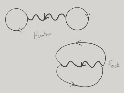
corresponding to the different ways of pairing the operators. Some of the diagrams arising at the second term in \(\eqref{Z_exp}\) are shown below
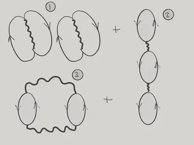
We see that some of these diagrams consist of a single connected component of interaction vertices joined by lines corresponding to pairing of creation and annihilation operators. The other diagrams consists of two disconnected copies of those that have already appeared at first order. The contribution from a diagram consisting of disconnected components factorizes, so there’s no difficulty including these repeated components as we will have already calculated them at a lower order in the series.
Now, what we actually want to calculate is not the partition function, but its logarithm, or derivatives thereof. For example,
\[ F = -k_\text{B}T \log Z \]
is the free energy, while
\[ U = -\frac{\partial}{\partial \beta}\log Z \]
is the internal energy. Fortunately, we have the following amazing fact, known as the linked cluster theorem:
The expansion of \(\log Z\) involves only those diagrams forming a single connected component .
Summing the Singular Diagrams
Let’s see how this works by evaluating the second order contribution to the free energy. According to the linked cluster theorem, this involves the diagrams
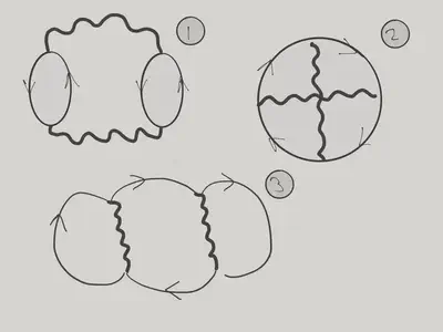
For Coulomb interactions, the first of these causes the biggest headache. To see what the problem is, let’s first write out the contribution of this diagram using Wick’s theorem.
\[ \begin{align} \frac{1}{8} \int_0^\beta d\tau_2 \int_0^{\beta} d\tau_1 \int \prod_{i=1}^4 d\br_i U(\br_1-\br_2)U(\br_3-\br_4)\nonumber\\ \times\pi(\br_4-\br_1,\tau_2-\tau_1)\pi(\br_2-\br_3,\tau_1-\tau_2), \label{2bubb} \end{align} \]
where \(\pi(\br,\tau)\) is the polarization
\[ \pi(\br,\tau) \equiv -\langle T_\tau \left(\rho(\br,\tau)-n\right)\left(\rho(0,0)-n\right)\rangle = G(\br,\tau)G(-\br,-\tau). \]
Writing \(\eqref{2bubb}\) in terms of momentum and frequency gives
\[ \begin{align} 2\times \frac{1}{8}\sum_{\bq,\omega_n} U_\bq^2\pi_{\bq,\omega_n}^2. \end{align} \]
The factor of \(2\) arises from the two ways in which one can pair the operators to get such a diagram.
Since \(U_\bq = \frac{4\pi e^2}{\abs{\bq}^2}\), we can see that – unless the behaviour of \(\pi_{\bq,\omega_n}\) saves us – these integrands will contain infrared divergences. Furthermore, higher order ring diagrams have even worse divergences!
There’s no sense in which these higher order diagrams are negligible. Fortunately, there’s a simple way to sum all diagrams of this class. Pairing operators to get a ring of \(p\) bubbles can be done in \(2^{p-1}(p-1)!\) ways. To see this, fix one of the factors of \(H_\text{int}\), and then choose one of the \((n-1)\) factors to pair with it. There are two ways to do it - depending on whether we pair with the top or bottom. Continuing this process gives the factor \(2^{p-1}(p-1)!\).
In this way we find the overall contribution to \(\log Z\)
\[ \begin{align} \sum_{p=1}^\infty\sum_{\bq,\omega_n}\frac{ 2^{p-1}(p-1)!}{2^p p!} \left[U_\bq \pi_{\bq,\omega_n}\right]^p =-\frac{1}{2}\sum_{\bq,\omega_n}\log\left[1-U_\bq \pi_{\bq,\omega_n}\right]. \end{align} \]
In this calculation we have taken into account only the contribution of the simplest diagram at each order with the highest singularity. Higher order diagrams can be interpreted as giving rise to a corrected polarization.
The physical meaning of this sum becomes clear if we consider the effect on the partition function of introducing some non-uniformity into the background charge density: \(n\to n+\delta n(\br)\). At first order in the interaction we obtain a rather trivial contribution to the free energy, arising from the interaction of this charge distribution with itself
\[ \frac{1}{2}\int d\br_1 d\br_2 \delta n(\br_1)U(\br_1-\br_2)\delta n(\br_2) = \frac{1}{2}\sum_\bq \delta n_\bq U_\bq \delta n_{-\bq}. \label{inhomog} \]
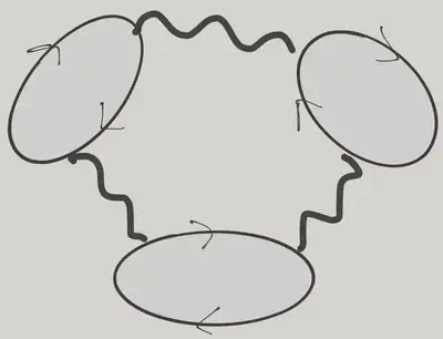
The above argument shows, however, that we cannot neglect the effect of the bubble diagrams, which now form a chain:
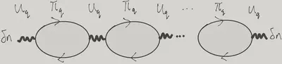
The combinatoric factor here is \(2^p p!\) at \(p^\text{th}\) order, showing that we now have a geometric series, rather than a logarithm. The overall effect is that at second order in \(\delta n(\br)\), the change in the free energy is still given by \(\eqref{inhomog}\), but now with the effective interaction
\[ U_{\text{eff},\bq} = \frac{U_\bq}{1-U_\bq \pi_{\bq,0}}. \]
The denominator can be interpreted as a dielectric function that tells us how the fermions modify the interaction between charges.
\[ \varepsilon(\bq,\omega_n) \equiv 1-U_\bq \pi_{\bq,\omega_n}. \label{dielectric} \]
It remains to calculate the polarization.
Evaluating the Polarization
In momentum and frequency space we have
\[ \pi_{\bq,\omega_n} = \frac{1}{\beta V}\sum_{\bp,\epsilon_m} G_{\bp+\bq,\epsilon_m+\omega_n}G_{\bp,\epsilon_m}. \label{pol} \]
Recall that \(\epsilon_m = 2\pi\left(m+\frac{1}{2}\right) T\) for fermions, while \(\omega_n\), being a sum of two fermionic Matsubara frequencies, is \(\omega_n = 2\pi n T\).
The sum in \(\eqref{pol}\) can be turned into an integral using the following neat formula
\[ \sum_{\epsilon_n} f(i\epsilon_n)=-i\frac{\beta}{4\pi }\int_\cC \tanh\left(\frac{\beta\epsilon}{2}\right)f(\epsilon) d\epsilon, \label{MatsubaraSum} \]
where the contour \(\cC\) encircles anti-clockwise only the poles of \(\tanh\left(\frac{\beta\epsilon}{2}\right)\), which lie at \(i\epsilon_n\). The formula then follows from finding the residues.
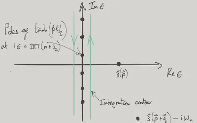
After writing \(\eqref{pol}\) as an integral, we can take the contour \(\cC\) to encircle clockwise the other poles of the integral, arising from the pair of Green’s functions, considered as functions of \(\epsilon\)
\[ G_{\bp,-i\epsilon}G_{\bp+\bq,\omega_n-i\epsilon} = \frac{1}{\left[\xi(\bp)-\epsilon\right]\left[\xi(\bp+\bq)-\epsilon-i\omega_n\right]}. \]
This then gives for the polarization
\[ \pi_{\bq,\omega_n} = \frac{1}{V}\sum_\bp \frac{\tanh\left(\frac{\beta\xi(\bp)}{2}\right)-\tanh\left(\frac{\beta\xi(\bp+\bq)}{2}\right)}{\xi(\bp+\bq)-\xi(\bp)-i\omega_n}. \]
Although this is still a complicated looking function, there are a couple of simple limits we can consider. We quote these, leaving their proof as an exercise
Static limit. \(\omega,\bk\to 0\), with \(\abs{\omega_n}\ll k_\text{F}\abs{\bq}/m\).
\[ \pi_{\bq,\omega}\to -\nu(E_\text{F}) \]
where \(\nu(E_F)\) is the density of states at the Fermi surface. This gives the effective interaction.
\[ U_{\text{eff},\bq} = \frac{U_\bq}{1+U_\bq \nu(E_\text{F})}, \]
which in real space has the formula
\[ U_\text{eff}(\br) = \frac{e^2}{\abs{\br}}\exp\left(-\abs{\br}/\lambda_\text{TF}\right), \]
where \(\lambda_\text{TF}=\sqrt{4\pi e^2\nu(E_F)}\) is the Thomas–Fermi screening length. Our summation of an infinite series of diagrams that are increasingly singular due to the long ranged nature of the Coulomb force is … a finite ranged potential!
High frequencies. \(\abs{\omega_n}\gg k_\text{F}\abs{\bq}/m\).
\[ \pi_{\bq,\omega_n} \longrightarrow -\frac{n\bq^2}{m\omega_n^2} \]
If we continue to real frequencies \(i\omega_n\to \omega + i0\), we find that in this limit the dielectric function in \(\eqref{dielectric}\) becomes
\[ \varepsilon(\bq,\omega) = 1-\frac{\omega_\text{p}^2}{\omega^2} \]
where \(\omega_\text{p}= \frac{4\pi e^2n}{m}\) is the plasma frequency. Reproducing this piece of classical physics is only possible because of the infinite summation we have performed.