\[ \nonumber \newcommand{\cN}{\mathcal{N}} \newcommand{\cH}{\mathcal{H}} \newcommand{\cC}{\mathcal{C}} \newcommand{\br}{\mathbf{r}} \newcommand{\bx}{\mathbf{x}} \newcommand{\bp}{\mathbf{p}} \newcommand{\bk}{\mathbf{k}} \newcommand{\bq}{\mathbf{q}} \newcommand{\bv}{\mathbf{v}} \newcommand{\pop}{\psi^{\vphantom{\dagger}}} \newcommand{\pdop}{\psi^\dagger} \newcommand{\Pop}{\Psi^{\vphantom{\dagger}}} \newcommand{\Pdop}{\Psi^\dagger} \newcommand{\Phop}{\Phi^{\vphantom{\dagger}}} \newcommand{\Phdop}{\Phi^\dagger} \newcommand{\phop}{\phi^{\vphantom{\dagger}}} \newcommand{\phdop}{\phi^\dagger} \newcommand{\aop}{a^{\vphantom{\dagger}}} \newcommand{\adop}{a^\dagger} \newcommand{\bop}{b^{\vphantom{\dagger}}} \newcommand{\bdop}{b^\dagger} \newcommand{\cop}{c^{\vphantom{\dagger}}} \newcommand{\cdop}{c^\dagger} \newcommand{\bra}[1]{\langle{#1}\rvert} \newcommand{\ket}[1]{\lvert{#1}\rangle} \newcommand{\inner}[2]{\langle{#1}\rvert #2 \rangle} \newcommand{\braket}[3]{\langle{#1}\rvert #2 \lvert #3 \rangle} \newcommand{\sgn}{\mathrm{sgn}} \newcommand{\brN}{\br_1, \ldots, \br_N} \newcommand{\xN}{x_1, \ldots, x_N} \newcommand{\zN}{z_1, \ldots, z_N} \newcommand{\abs}[1]{\lvert{#1}\rvert} \]
The Kondo model describes a single spin coupled to a Fermi gas. It seems innocuous enough: one small step up in difficulty from a static impurity, perhaps. Not so! The Kondo problem has in fact played a huge role in many body physics over the years, both for the methods required to solve it, and because it keeps popping up in different guises.
Reading: {% cite Kouwenhoven:2001aa %}, {% cite Hewson:1997aa %}, {% cite Kondo:2012aa %},
The Kondo Model
Jun Kondo’s paper Resistance Minimum in Dilute Magnetic Alloys presents a theoretical solution to a puzzling, but perhaps unspectacular observation. At low temperatures, the resistance of metals falls. This is nothing to do with superconductivity, but is a more mundane consequence of electron-electron or electron-phonon scattering falling with temperature, as the thermal population of phonons or particle hole pairs diminishes. Evidence had accumulated over the years, however, that in nonmagnetic metals containing magnetic impurities (Copper with Manganese or Iron, for example), the low temperature resistance eventually began to rise again.
The fact that the effect could be observed with tiny concentrations of magnetic impurities (as low as 0.0005% Iron atoms in Copper!), lead Kondo to study the scattering of electrons by single impurity, described by the model that now bears his name
\[ H = \sum_{\bk,s=\uparrow,\downarrow} \xi(\bk)\adop_{\bk,s}\aop_{\bk,s} + \overbrace{J \mathbf{S}\cdot \mathbf{s}(0)}^{\equiv H_J} \label{Kondo} \]
The first term is just the kinetic energy of free fermions, while the second describes the coupling of an impurity spin \(\mathbf{S}\) – which we will take to be \(S=1/2\), though of course other values are possible – to the spin density of the fermions
\[ \mathbf{s}(\br)= \sum_{s,s'}\pdop_{s}(0)\frac{\boldsymbol{\sigma}_{ss'}}{2}\pop_{s'}(0)=\frac{1}{V}\sum_{\substack{\bk,\bk'\\s,s'}} \frac{\boldsymbol{\sigma}_{ss'}}{2}\adop_{k',s'}\aop_{k,s}. \]
The fermions and impurity are coupled at the origin, where the impurity is assumed to be located.
Kondo showed that, unlike nonmagnetic impurities, which give rise to temperature independent scattering and to the residual resistance of metals, scattering from a magnetic impurity was enhanced at low energies or temperatures. His perturbation theory calculation, which we’ll repeat below, gave a correction to the scattering, and hence to the resistivity, proportional to \(\log T\). This was as observed in experiment.
It all looked good, except that – and this is where the emphasis shifted strongly to the theoretical aspects of the problem – this contribution to the scattering was diverging as the energy of the scattered fermion vanished. In a practical sense, that meant that Kondo’s calculation could not be trusted at energies where the correction becomes large. The more conceptual issue was: what did it mean? What was the spin of the impurity doing to the Fermi sea?
The Kondo model went on to become one of the testbeds of the renormalization group (RG) approach to many body physics, quantum field theory, and statistical mechanics. The RG is a framework for understanding the behaviour of systems at scales intermediate between the microscopic (Fermi wavelength or size of impurity in this case) and the macroscopic (size of the system). The idea is that is that if these scales are separated by many orders of magnitude, the behaviour at intermediate scales should be approximately scale independent. In the case of the Kondo model, the effective Hamiltonians (we met this notion in Lecture 7 ) at different energy scales should be almost the same. The incompleteness of the scale invariance is encoded in a variation of the parameters of the effective Hamiltonian.
In this context, the divergences found by Kondo in his perturbative calculation can be understand as a finite renormalization of the parameters of the effective Hamiltonian as the scale changes. We will see how this point of view allows us to understand the low energy behaviour of the Kondo model in much greater detail. The utility of the RG is not restricted to perturbation theory, but this is all we’ll have time for.
Kondo’s Calculation
We are going to consider the scattering of a single fermion above the Fermi sea, described by the state
\[ \ket{\bk,s}\equiv \adop_{\bk,s}\ket{\text{FS}}\otimes \ket{S}_\text{imp}, \]
where \(\ket{\text{FS}}\) is the Fermi sea ground state of the Fermi gas, and \(\ket{S}_\text{imp}\) describes the spin. In time dependent perturbation theory in the coupling between the impurity and the fermions we compute the scattering amplitude by expanding the interaction picture evolution operator
\[ U_\text{I}(t)=T \exp\left(-i\int_0^t H_J(t') dt'\right), \]
where \(T\) denotes time ordering, and the time evolution of the coupling is
\[ H_J(t) = \frac{J}{V}\sum_{\substack{\bk,\bk'\\s,s'}} \mathbf{S}(t)\cdot\frac{\boldsymbol{\sigma}_{ss'}}{2}\adop_{k',s'}(t)\aop_{k,s}(t), \]
with
\[ \aop_{\bk,s}(t) = e^{-i\xi(\bk)t}\aop_{\bk,s},\quad \adop_{\bk,s}(t) = e^{i\xi(\bk)t}\adop_{\bk,s}. \]
\(\mathbf{S}(t)\) has no time dependence since the impurity spin does not appear in the unperturbed Hamiltonian. Nevertheless, we label it so as to keep track of the order in which it appears, coupled to operators with true time dependence, when we expand the evolution operator.
First Order
At first order \(H_J\) can create a particle hole pair or scatter the particle. We are considering scattering, so we consider initial and final states of the form
\[ \ket{\bk,s,S}\equiv\adop_{\bk,s}\ket{\text{FS}}\otimes \ket{S}_\text{imp}. \]
The relevant matrix element is just
\[ \begin{align} -i\braket{\bk,s,S}{H_J(t)}{\bk',s',S'} &=-i\frac{J}{4V}\boldsymbol{\sigma}_{SS'}\cdot\boldsymbol{\sigma}_{ss'}e^{i[\xi(\bk)-\xi(\bk')]t}. \label{1stAmp} \end{align} \]
The Fermi Golden Rule then gives the scattering rate
\[ \Gamma_{\bk',s',S'\to \bk,s,S} = 2\pi\left(\frac{J}{4V}\right)^2\abs{\boldsymbol{\sigma}_{SS'}\cdot\boldsymbol{\sigma}_{ss'}}^2\delta(\xi(\bk)-\xi(\bk')). \]
Summing over final states gives
\[ \begin{align} \Gamma^{\text{1 imp}}_{\bk',s',S'} &=\sum_{\bk,s,S} \Gamma_{\bk',s',S'\to\bk,s,S}\nonumber\\ &=V\sum_{s,S}\int \nu(\xi) \Gamma_{\bk',s',S'\to\bk ,s,S}d\xi\nonumber\\ &=\frac{\pi J^2\nu(\xi)}{2V}\left(5-4\delta_{s'S'}\right) \end{align} \]
where \(\nu(\xi)\) is the density of states per spin component per unit volume. When \(S'\neq s'\) the scattering is larger because spin flip processes are allowed as well as those that don’t flip the spin.
If we add up the scattering for a dilute concentration of impurities \(n_\text{imp}\) by simply multiplying by their number \(N_\text{imp}=n_\text{imp}V\) and averaging over the initial spin orientation, we get
\[ \Gamma = \frac{3\pi n_\text{imp}J^2\nu(\xi)}{2} \]
Second Order
The magic happens at the next order, where we have the contribution to the amplitude
\[ \begin{align} -\int_0^t dt_2 \int_0^{t_2}dt_1\braket{\bk,s,S}{H_J(t_2)H_J(t_1)}{\bk',s',S'}. \end{align} \]
Comparing with the first order amplitude \(\eqref{1stAmp}\) shows that
\[ \begin{align} - \int_0^{t}dt'\braket{\bk,s,S}{H_J(t)H_J(t')}{\bk',s',S'}, \end{align} \]
can be regarded as a correction to the matrix element to be inserted into the Golden Rule.
If we insert a complete set of states between the two occurrences of \(H_J\), what intermediate (or virtual) states contribute to the scattering amplitude? There are just two possibilities
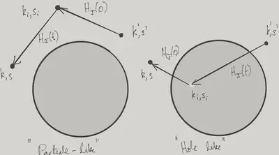
The fermion scatters to \(\bk_i\), \(s_i\), with \(\bk_i\) above the Fermi surface.
A particle hole pair is created, with the particle at \(\bk,s\). The hole is subsequently filled.
We see that indistinguishability (and hence fermionic statistics) plays a fundamental role in the second process.
We consider the particle process first. This arises from the terms
\[ \begin{align} H_J(t') &\longrightarrow \frac{J}{4V} \boldsymbol{\sigma}_{S_iS'}\cdot \boldsymbol{\sigma}_{s_i s'}\adop_{\bk_i,s_i}(t')\aop_{\bk',s'}(t')\nonumber\\ H_J(t) &\longrightarrow \frac{J}{4V} \boldsymbol{\sigma}_{SS_i}\cdot \boldsymbol{\sigma}_{ss_i}\adop_{\bk,s}(t)\aop_{\bk_i,s_i}(t),\quad \abs{\bk_i}>k_\text{F} \end{align} \]
The time dependence of the operators gives rise to the phase factor
\[ \begin{align} \exp\left(i[\xi(\bk)-\xi(\bk_i)]t+i[\xi(\bk_i)-\xi(\bk')]t'\right)\nonumber\\ = \exp\left(i[\xi(\bk)-\xi(\bk')]t+i[\xi(\bk_i)-\xi(\bk')](t'-t)\right) \end{align} \]
Extending the integral over \(t-t'\) to \(\infty\) gives
\[ \int_0^\infty d(t-t') \exp\left(i[\xi(\bk')-\xi(\bk_i)](t-t')\right) = \frac{i}{\xi(\bk')-\xi(\bk_i)+i0}. \]
Putting it all together gives a contribution
\[ -i\sum_{\abs{\bk_i}>k_\text{F}}\frac{\exp\left(i[\xi(\bk)-\xi(\bk')]t\right)}{\xi(\bk')-\xi(\bk_i)+i0}\left(\frac{J}{4V}\right)^2\left(\sigma^j\sigma^k\right)_{SS'}\left(\sigma^j\sigma^k\right)_{ss'}. \label{plike} \]
Now we turn to the hole process. The relevant terms in the coupling are now
\[ \begin{align} H_J(t') &\longrightarrow \frac{J}{4V} \boldsymbol{\sigma}_{S_iS'}\cdot \boldsymbol{\sigma}_{s s_i}\adop_{\bk,s}(t')\aop_{\bk_i,s_i}(t')\nonumber\\ H_J(t) &\longrightarrow \frac{J}{4V} \boldsymbol{\sigma}_{SS_i}\cdot \boldsymbol{\sigma}_{s_i s'}\adop_{\bk_i,s_i}(t)\aop_{\bk',s'}(t),\quad \abs{\bk_i}<k_\text{F}. \end{align} \]
The phase factor is now
\[ \begin{align} \exp\left(i[\xi(\bk_i)-\xi(\bk')]t+i[\xi(\bk)-\xi(\bk_i)]t'\right)\nonumber\\ = \exp\left(i[\xi(\bk)-\xi(\bk')]t+i[\xi(\bk)-\xi(\bk_i)](t'-t)\right). \end{align} \]
Integrating over \(t-t'\) then gives
\[ \int_0^\infty d(t-t') \exp\left(i[\xi(\bk_i)-\xi(\bk)](t-t')\right) = \frac{i}{\xi(\bk_i)-\xi(\bk)+i0}. \]
On account of the order of \(\adop_{\bk,s}\) and \(\aop_{\bk',s'}\) being reversed, we have a minus sign relative to the particle contribution, leading to
\[ i\sum_{\abs{\bk_i}<k_\text{F}}\frac{\exp\left(i[\xi(\bk)-\xi(\bk')]t\right)}{\xi(\bk_i)-\xi(\bk)+i0}\left(\frac{J}{4V}\right)^2\left(\sigma^j\sigma^k\right)_{SS'}\left(\sigma^k\sigma^j\right)_{ss'}. \label{hlike} \]
The phase factors in \(\eqref{plike}\) and \(\eqref{hlike}\), as in the first order result \(\eqref{1stAmp}\), are responsible for the \(\delta\)-function setting \(\xi(\bk)=\xi(\bk')\) in the Golden Rule. Both \(\eqref{plike}\) and \(\eqref{hlike}\) have a logarithmic divergence that is cut-off at low energies by \(\xi(\bk)=\xi(\bk')\). For example,
\[ \sum_{\abs{\bk_i}>k_\text{F}}\frac{1}{\xi(\bk')-\xi(\bk_i)+i0}\sim -\nu(0)V\log\left(\frac{\Lambda}{\xi(\bk)}\right), \]
where \(\Lambda\) is an upper cut-off arising from the microscopic scales of the problem. The overall logarithmic dependence of the second order correction is then
\[ i\frac{J^2\nu(0)}{32 V}\exp\left(i[\xi(\bk)-\xi(\bk')]t\right)\log\left(\frac{\Lambda}{\xi(\bk)}\right)\left[\sigma^j,\sigma^k\right]_{SS'} \left[\sigma^j,\sigma^k\right]_{ss'}. \label{TotalLog} \]
Since
\[ \left[\sigma^j,\sigma^k\right]_{SS'} = 2i\epsilon_{jkl} \sigma^l_{SS'}, \]
we can interpret \(\eqref{TotalLog}\) as a logarithmic correction to the coupling \(J\)
\[ \delta J = \frac{J^2\nu(0)}{2}\log\left(\frac{\Lambda}{\xi(\bk)}\right). \label{KondoCorrect} \]
This was Kondo’s discovery. For \(J>0\) this represents an increase in the magnitude of the coupling, and a corresponding logarithmic correction to the scattering rate. At finite temperature, the lower cutoff in the integrals is replaced by the temperature, leading to the observed \(\log T\) dependence of the resistivity on temperature.
It’s instructive to compare this calculation with what you would get for a static impurity described by a localized potential. We know that this situation could be described by solving the single particle problem including the potential and just filling the resulting states. The appearance of the spin commutation relations in \(\eqref{TotalLog}\) shows us that the quantum dynamics of the impurity is essential.
Renormalization Group analysis of the Kondo Hamiltonian
The logarithmic correction \(\eqref{KondoCorrect}\) becomes the same order as \(J\) when the low energy cut-off approaches the Kondo scale
\[ E_\text{K} \equiv \Lambda \exp\left(-\frac{2}{\nu(0)\abs{J}}\right). \]
What can we say about the physics at or below this scale? Continuing with perturbation theory leads to contributions \(\propto \log^p(\Lambda/\xi)\) with \(p>1\), which doesn’t really help to clarify things. An alternative is to ask for the effective Hamiltonian describing the problem on a particular scale.
Effective Hamiltonian
To be precise, we start with a Kondo problem defined with a certain \(\Lambda\). Then, for \(\Lambda'\ll\Lambda\), we ask for the effective Hamiltonian describing the system when there are no particle excitations with \(\xi(\bp)>\Lambda'\) and no hole excitations with \(\xi(\bp)<-\Lambda'\). Let’s refer to this subspace as \(\cH_{\Lambda'}\). This effective Hamiltonian is different from the original Hamiltonian: we saw in Lecture 7 that, since \(\Lambda'\ll \Lambda\), the effective Hamiltonian in \(\cH_{\Lambda'}\) is
\[ \delta H = - H_JP_{[\Lambda',\Lambda]}H_0^{-1}H_J, \]
where \(P_{[\Lambda',\Lambda]}\) projects on particle excitations with \(\Lambda>\xi(\bp)>\Lambda'\) and hole excitations with \(-\Lambda<\xi(\bp)<-\Lambda'\). It’s not hard to see that evaluating \(\delta H\) is very similar to the second order calculation of the previous section, showing that \(\delta H\) has the same form as \(H_J\) with \(\delta J\) given by
\[ \delta J = \frac{J^2\nu(0)}{2}\log\left(\frac{\Lambda}{\Lambda'}\right). \label{KondoCorrectRG} \]
The implication is that the physics of excitations within \(\Lambda'\) of the Fermi surface can be described either by the original Hamiltonian with cut-off \(\Lambda\), or by \(H+\delta H\) – the same model with \(J\to J+\delta J\) – with cut-off \(\Lambda'\).
Scaling of the Hamiltonian
Now let’s see what this has to do with scale invariance. Suppose we were studying the Kondo problem in which we had already removed almost all the degrees of freedom, leaving only those in a thin shell of energy thickness \(2\Lambda\) around the Fermi surface
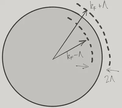
The Kondo model defined in this shell may be written
\[ \begin{align} \frac{H_\Lambda}{V} &= \nu(0)\sum_s\int_{-\Lambda}^\Lambda d\xi \int_{S^2} d\Omega_{\hat{\mathbf{n}}}\,\xi \adop_{\bk,s}\aop_{\bk,s}\nonumber \\ &+\nu(0)^2J \mathbf{S}\cdot \int_{-\Lambda}^\Lambda d\xi \int_{-\Lambda}^\Lambda d\xi' \int_{S^2} d\Omega_{\hat{\mathbf{n}}} \int_{S^2}d\Omega_{\hat{\mathbf{n}}'} \sum_{s,s'}\frac{\boldsymbol{\sigma}_{ss'}}{2} \adop_{\bk,s}\aop_{\bk',s'} \label{KondoShell} \end{align} \]
where
\[ \bk = \hat{\mathbf{n}} \left(k_\text{F}+ \xi/v_\text{F}\right),\quad \bk' = \hat{\mathbf{n}}' \left(k_\text{F}+ \xi/v_\text{F}\right). \]
Now, \(\eqref{KondoShell}\) has the feature that both terms scale the same way under a re-scaling \(\Lambda\to\Lambda'\), essentially because both contain the second power of \(\xi\).
To state this more precisely, let’s re-define the field operators to incorporate factors of \(\sqrt{V}\)
\[ \adop_{\hat{\mathbf{n}},\xi,s}\equiv \sqrt{V}\adop_{\bk,s},\quad \aop_{\hat{\mathbf{n}},\xi,s}\equiv \sqrt{V}\aop_{\bk,s},\quad \]
so now
\[ \begin{align} \left\{\aop_{\hat{\mathbf{n}},\xi,s},\adop_{\hat{\mathbf{n}}',\xi',s'}\right\}=(2\pi)^3\delta_{ss'}v_\text{F} k_\text{F}^{-2}\delta(\hat{\mathbf{n}}-\hat{\mathbf{n}}')\delta(\xi-\xi'), \label{CARcont} \end{align} \]
and
\[ \begin{align} H_\Lambda&= \nu(0)\sum_s\int_{-\Lambda}^\Lambda d\xi \int_{S^2} d\Omega_{\hat{\mathbf{n}}}\,\xi \adop_{\hat{\mathbf{n}},\xi,s}\aop_{\hat{\mathbf{n}},\xi,s} \nonumber \\ &+\nu(0)^2J \mathbf{S}\cdot \int_{-\Lambda}^\Lambda d\xi \int_{-\Lambda}^\Lambda d\xi' \int_{S^2} d\Omega_{\hat{\mathbf{n}}} \int_{S^2}d\Omega_{\hat{\mathbf{n}}'} \sum_{s,s'}\frac{\boldsymbol{\sigma}_{ss'}}{2} \adop_{\hat{\mathbf{n}},\xi,s}\aop_{\hat{\mathbf{n}}',\xi',s'}. \label{KondoShellInfinite} \end{align} \]
In this way, we can state the scaling of the Hamiltonian precisely as
\[ H_\Lambda(\adop_{\hat{\mathbf{n}},\xi,s},\aop_{\hat{\mathbf{n}},\xi,s}) =\frac{\Lambda}{\Lambda'} H_{\Lambda'}\left(\tilde\adop_{\hat{\mathbf{n}},\xi,s},\tilde\aop_{\hat{\mathbf{n}},\xi,s}\right) \label{Hscale} \]
where
\[ \tilde\adop_{\hat{\mathbf{n}},\xi,s} = \sqrt{\frac{\Lambda}{\Lambda'}}\adop_{\hat{\mathbf{n}},\frac{\Lambda}{\Lambda'}\xi,s},\quad \tilde\aop_{\hat{\mathbf{n}},\xi,s} = \sqrt{\frac{\Lambda}{\Lambda'}}\aop_{\hat{\mathbf{n}},\frac{\Lambda}{\Lambda'}\xi,s} \]
obey the same relations \(\eqref{CARcont}\).
\(\eqref{Hscale}\) is inarguable as an operator identity between Kondo Hamiltonians defined in two different energy shells. However, the previous section shows that the effective Hamiltonian acting in the \(\Lambda'\) (sub-)shell for a system described by \(H_\Lambda\) in the \(\Lambda\) shell is not \(H_{\Lambda'}\), but \(H_{\Lambda'}+\delta H\). Thus the similarity between the two scales is incomplete, but can be fixed by the modest change
\[ \delta J = \frac{J^2\nu(0)}{2}\log\left(\frac{\Lambda}{\Lambda'}\right). \]
Having returned to the original \(\Lambda\) shell, with only a shift in the coupling to show for it (and an overall scaling in the Hamiltonian – see \(\eqref{Hscale})\), we are free to repeat the procedure again. In this way the renormalization of \(J\) is iterated repeatedly. Normally, we express this iteration not in terms of a discrete mapping of the coupling of the Hamiltonian, but through a differential equation.
\[ \frac{dJ}{d\tau} = \frac{J^2\nu(0)}{2} \label{RGIso} \]
where \(\tau\equiv\log \Lambda/\Lambda'\) represents the scale factor between the original scale \(\Lambda\) and the current scale \(\Lambda'\).
There’s something a bit fishy about this last step. After all, wasn’t the effective Hamiltonian derived on the assumption that \(\Lambda'\ll \Lambda\)? Thinking in differential terms really only requires \(J\nu(0)\Delta t\ll 1\), however, which can be satisfied even if \(\Lambda\gg\Lambda'\).
is an example of an RG flow equation, expressing the incomplete self-similarity of the Kondo problem as we zoom inwards ever closer to the Fermi surface. Similar equations describe the scaling of parameters in theories describing continuous phase transitions – where there are fluctuations at all length scales – or massless quantum field theories – where zero mass means the absence of any length or timescale.
Solution of the RG Equations
The single equation \(\eqref{RGIso}\) is a bit boring. We can make things more interesting by introducing anisotropy into the original Kondo coupling
\[ H_J = \frac{1}{V}\sum_{\substack{\bk,\bk'\\ s,s'}} \left[J_\parallel S^z s^z_{ss'}\adop_{k',s'}\aop_{k,s} + J_\perp\left( S^+\frac{s^-_{ss'}}{2}\adop_{k',s'}\aop_{k,s} +\text{h.c.}\right)\right]. \]
It isn’t hard to show that \(\eqref{RGIso}\) is now replaced with
\[ \begin{align} \frac{dJ_\parallel}{d\tau} &= \frac{J_\perp^2\nu(0)}{2}\nonumber\\ \frac{dJ_\perp}{d\tau} &= \frac{J_\perp J_\parallel\nu(0)}{2}. \end{align} \]
The character of the solutions can be readily understood by noticing that
\[ J_\perp^2-J_\parallel^2=\text{const.} \]
is preserved along the flow, leading to a series of hyperbolae. It remains to figure out the direction of the flow:
](/courses/tqm/kondo-effect/AndersonRG_hud9167cb0c6b82f1594755cac550f44ab_34409_ac37469cc435e8e85eb5dded42702432.webp)
The conclusions of this analysis are as follows:
For ferromagnetic couplings \(J_z<0\) with \(\abs{J_z}>\abs{J_\perp}\), the flow is to \(J_\perp=0\). This means that at low energies the amplitude for spin-flips vanishes, leaving only a \(S^z s^z(0)\) coupling.
For antiferromagnetic coupling \(J_z>0\), or ferromagnetic coupling with \(\abs{J_z}<\abs{J_\perp}\), the flow is to strong coupling. This means that our analysis – which was still based on the smallness of \(J\) despite all the fancy bells and whistles – breaks down.
It would be remiss of me not to mention that exactly the same RG flow governs the Kosterlitz–Thouless transition of two dimensional superfluid systems, cited in the 2016 Nobel Prize. In this case the role of \(J_\parallel\) is taken by the deviation in temperature from the critical temperature, and \(J_\perp\) corresponds to the chemical potential of vortices, which proliferate at the transition.
Epilogue: What Really Happens?
My intention in this lecture was to give a taste of what makes the Kondo problem so intriguing. However, we certainly haven’t gotten to the bottom of it. Let me try to summarize an enormous amount of history in a paragraph or two.
Kenneth Wilson’s numerical RG calculations, which informed his formulation of the general framework that won him the Nobel prize, showed that in the low energy limit the impurity spin is completely ‘quenched’, forming a singlet with the Fermi sea {% cite Wilson:1975aa %}. This is a highly nontrivial process, but a simple caricature is that the singlet forms with the one fermion allowed at the site of the impurity by the exclusion principle. This process is often called screening in analogy to a plasma, though the physics is of course rather different. Nevertheless, it leads to a very simple Fermi liquid-like picture of the physics close to the ground state, as explained by Nozières {% cite Nozieres:1974aa %}
The same qualitative consideration lets us understand what happens for larger impurity spin \(S\): in the ground state the impurity has spin \(S-1/2\). We can also add more ‘channels’, coupling the impurity to other species of fermions that represent the interaction of different partial waves (angular momentum states) with the impurity. Then it is possible for ‘overscreening’ to occur, meaning that the strongly coupled picture is unstable as both channels try to form a singlet with the impurity. The instability of both strong and weak coupling suggests an intermediate coupling ground state, which turns out to have highly unusual non-Fermi liquid properties without well defined fermionic quasiparticles. However, this state only exists for exactly equal coupling in two or more channels, which is unlikely to occur with a magnetic impurity atom.
One of the great innovations of the last couple of decades is the use of quantum dots as artificial magnetic impurities. These mesoscopic electronic devices can be connected in a circuit, so that the Kondo effect is probed by electical conduction rather than through the resistivity that arises from scattering. Even better, quantum dots are a a highly tunable Kondo system that has allowed the two-channel effect to be observed, for example. You can read about some of these developments in the article {% cite Kouwenhoven:2001aa %}.
You can find even more in the textbook {% cite Hewson:1997aa %} or {% cite Kondo:2012aa %} from the man himself.
References
{% bibliography –cited %}