Lieb-Liniger Model

\[ \nonumber \newcommand{\cN}{\mathcal{N}} \newcommand{\cC}{\mathcal{C}} \newcommand{\br}{\mathbf{r}} \newcommand{\bx}{\mathbf{x}} \newcommand{\bp}{\mathbf{p}} \newcommand{\bk}{\mathbf{k}} \newcommand{\bq}{\mathbf{q}} \newcommand{\bv}{\mathbf{v}} \newcommand{\pop}{\psi^{\vphantom{\dagger}}} \newcommand{\pdop}{\psi^\dagger} \newcommand{\Pop}{\Psi^{\vphantom{\dagger}}} \newcommand{\Pdop}{\Psi^\dagger} \newcommand{\Phop}{\Phi^{\vphantom{\dagger}}} \newcommand{\Phdop}{\Phi^\dagger} \newcommand{\phop}{\phi^{\vphantom{\dagger}}} \newcommand{\phdop}{\phi^\dagger} \newcommand{\aop}{a^{\vphantom{\dagger}}} \newcommand{\adop}{a^\dagger} \newcommand{\bop}{b^{\vphantom{\dagger}}} \newcommand{\bdop}{b^\dagger} \newcommand{\cop}{c^{\vphantom{\dagger}}} \newcommand{\cdop}{c^\dagger} \newcommand{\bra}[1]{\langle{#1}\rvert} \newcommand{\ket}[1]{\lvert{#1}\rangle} \newcommand{\inner}[2]{\langle{#1}\rvert #2 \rangle} \newcommand{\braket}[3]{\langle{#1}\rvert #2 \lvert #3 \rangle} \newcommand{\sgn}{\mathrm{sgn}} \newcommand{\brN}{\br_1, \ldots, \br_N} \newcommand{\xN}{x_1, \ldots, x_N} \newcommand{\zN}{z_1, \ldots, z_N} \newcommand{\abs}[1]{\lvert{#1}\rvert} \]

In this lecture we are going to look at a model of many interacting particles that we can solve exactly. The price we pay is that the model is rather special: it describes particles moving in one dimension with short range interactions.

Reading: {% cite Sutherland:2004 %}.

The Model

In the first lecture we encountered the Hamiltonian

\[ H = -\frac{1}{2m}\sum_j \frac{\partial^2}{\partial x_j^2} + c\sum_{j<k}\delta(x_j-x_k), \label{LL_LL} \]

describing a system of interacting one dimensional bosons. We showed that the \(c\to\infty\) limit of this model can be described in terms of noninteracting fermions. We are now going to discuss the solution for general \(c\). This is possible because the eigenfunctions, which are not product states, have a very special form first written down by Hans Bethe in 1931 – so soon after the birth of quantum mechanics! – in the context of the Heisenberg model of a spin chain (see Lecture 4). Bethe’s approach was applied to the model \(\eqref{LL_LL}\) by Lieb and Liniger in 1963 {% cite Lieb:1963aa %}, and for that reason it is usually known as the Lieb–Liniger model.

Bethe’s Wavefunction

Bethe’s wavefunction – often known as the Bethe ansatz – can be viewed as the factorization of the scattering of the \(N\) particles in the gas into a sequence of two particle scattering events. The fact that this works is very special, and is restricted to one dimension. Furthermore, it only works for very special interaction potentials, of which the \(\delta\)-function is the simplest example.

Thus we start by considering the two particle problem.

Two Particles

The two particle time independent Schrödinger equation is

\[ \left[-\frac{1}{2}\left(\frac{\partial^2}{\partial x_1^2}+\frac{\partial^2}{\partial x_2^2}\right) + c\delta(x_1-x_2)\right]\Psi(x_1,x_2)=E\Psi(x_1,x_2), \label{LL_2part} \]

(We’ve set \(m=1\).) Since we are dealing with bosons \(\Psi(x_1,x_2) = \Psi(x_2,x_1)\). Away from \(x_1=x_2\) we have the free particle Schrödinger equation, so the general solution is a superposition of plane waves of the form

\[ \Psi(x_1,x_2) = \exp(i[k_1 x_1 + k_2 x_2]) \label{LL_1wave} \]

\(\eqref{LL_1wave}\) describes a state with momentum \(P_\text{tot}= k_1+k_2\) and energy \(E_\text{tot} = \frac{k_1^2}{2}+\frac{k_2^2}{2}\). Note that for given values of \(P_\text{tot}\) and \(E_\text{tot}\), the most general solution contains only the two terms

\[ \Psi(x_1,x_2) = A_{12} \exp(i[k_1 x_1 + k_2 x_2]) + A_{21} \exp(i[k_1 x_2 + k_2 x_1]),\quad x_1\leq x_2, \label{LL_Psi2} \]

with the solution extended to \(x_1>x_2\) by symmetry.

\[ \Psi(x_1,x_2) = A_{12} \exp(i[k_1 x_2 + k_2 x_1]) + A_{21} \exp(i[k_1 x_1 + k_2 x_2]),\quad x_1 \geq x_2. \label{LL_Psi2b} \]

The relationship between the amplitudes \(A_{12}\) and \(A_{21}\) is determined by the interaction. Substituting \(\eqref{LL_Psi2}\) into the Schrödinger equation \(\eqref{LL_2part}\) gives

\[ -i\left[A_{12}(k_2-k_1) + A_{21}(k_1-k_2)\right] + c\left[A_{12}+A_{21}\right]=0, \]

or

\[ \frac{A_{21}}{A_{12}} = \frac{k_1 - k_2 -ic}{k_1 - k_2 +ic} \equiv \exp\left[-i\theta(k_1-k_2)\right]. \]

The last equation defines the phase shift \(\theta(k)\). Note that conservation of flux and the symmetry of the wavefunction means that \(\abs{A_{12}}=\abs{A_{21}}\). In the impenetrable limit (\(c\to\infty\)) the phase shift goes to \(\pi\).

Three Particles

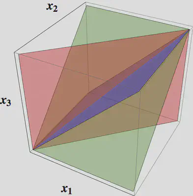
What about three particles? The wavefunction \(\Psi(x_1,x_2,x_3)\) can be pictured as a function in 3D space, with the interactions imposing conditions at the three planes \(x_1=x_2\), \(x_2=x_3\), and \(x_1=x_3\).

Away from these planes, we expect the wavefunction to be a superposition of plane waves of fixed energy

\[ \Psi_{\bk}(\bx) = \exp\left(i\bk\cdot\bx\right), \]

with \(\bk = (k_1,k_2,k_3)\) and \(\bx = (x_1,x_2,x_3)\). This describes a state with

\[ P_\text{tot} = k_1+k_2+k_3,\qquad E_\text{tot} = \frac{k_1^2}{2}+\frac{k_2^2}{2} + \frac{k_3^2}{2}. \]

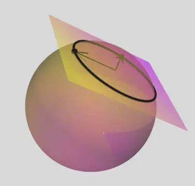
We can picture these conditions as the intersection of a plane and a sphere in momentum space. This illustrates that on kinematic grounds alone we should expect a continuum of plane waves in the superposition to make an eigenstate. It is here, however, that the special nature of the interaction saves us, as it turns out that can get away with only a finite superposition of all the \(3!=6\) ways to assign the three momenta \((k_1,k_2,k_3)\) to the three particles.

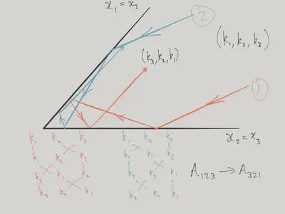
There is a nice geometrical picture that allows us to understand why this is. In the above 3D representation, the centre of mass coordinate of the three particles is increasing in the \((1,1,1)\) direction, in which the system naturally has translational invariance. The plane perpendicular to this direction describes the relative motion of the three particles. In this plane the three planes corresponding to the pairwise coincidence of particle coordinates appear as three lines at \(\pi/3\) to each other, meeting at the origin.

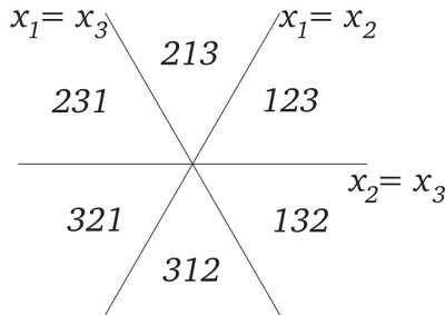
The plane is divided into six regions that correspond to the \(3!=6\) arrangements of the three particles on the line. Bosonic symmetry means that the wavefunction is the same in each of the six sectors. The scattering of three particles can then be viewed as a solution to the wave equation in 2D, with boundary conditions imposed by the interaction on the lines.

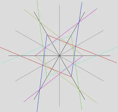
If we think of scattering in the classical limit – rays undergoing specular reflection from the mirrors of the kaleidoscope – then an incoming ray can only to scatter to five other directions, no matter which order it hits the walls. This collection of six rays corresponds to the six possible assignments of the three momenta \((k_1,k_2,k_3)\) to the three particles.

For the real wave problem this suggests that the wavefunction has the form

\[ \Psi(x_1,x_2,x_3) = \sum_P A_P \exp\left(i\sum_{j=1}^3 k_{P(j)}x_j\right),\quad x_1\leq x_2\leq x_3. \label{LL_3part} \]

With the amplitudes \(A_P\) chosen so as to satisfy the boundary conditions. However, we already know how to do this from our analysis of the two particle problem. We must have, for instance

\[ \frac{A_{213}}{A_{123}} = \exp\left[-i\theta(k_1-k_2)\right]. \]

In this way, you can convince yourself that

\[ \frac{A_{321}}{A_{123}} = \exp\left[-i\theta(k_1-k_2)-i\theta(k_2-k_3)-i\theta(k_1-k_3)\right] \]

irrespective of which transpositions of neighbouring momenta we used to get from \((123)\) to \((321)\). In terms of our kaleidoscope, this corresponds to different rays having the same phase, no matter in which order they hit the mirrors.

Bethe Ansatz for \(N\) Particles

The Bethe ansatz for \(N\) particles is a straightforward generalization of \(\eqref{LL_3part}\), and depends on a set of \(N\) momenta \(k_1,\ldots k_N\)

\[ \Psi(x_1,x_2,\ldots,x_N) = \sum_P A_P \exp\left(i\sum_{j=1}^N k_{P(j)}x_j\right),\quad x_1\leq x_2\leq\cdots x_N. \label{LL_Npart} \]

The momentum and energy are

\[ P_\text{tot} = \sum_{j=1}^N k_j,\qquad E_\text{tot} = \sum_{j=1}^N\frac{k_j^2}{2}. \]

I want to emphasize that, despite the apparent complexity of the wavefunction \(\eqref{LL_Npart}\), consisting of a sum over \(N!\) permutations, it represents a huge simplification over the most general superposition of plane wave states of fixed energy and momentum.

By considering the condition at \(x_j=x_{j+1}\) we obtain a relationship between \(A_P\) and \(A_{P'}\), where the permutations \(P\) and \(P'\) are related by the exchange of \(P(j)\) and \(P(j+1)\)

\[ P'=(P(1),P(2),\ldots, P(j-1),P(j+1),P(j),P(j+2),\ldots,P(N)). \]

The same analysis as for the two particle case yields

\[ \frac{A_{P'}}{A_P} = \frac{k_{P(j)}-k_{P(j+1)}-ic}{k_{P(j)}-k_{P(j+1)}+ic} = \exp\left[-i\theta(k_{P(j)}-k_{P(j+1)})\right]. \label{LL_NExchange} \]

It can be checked that a solution of the set of such equations is given by

\[ A_P = \prod_{1\leq j<k\leq N}\left(1 + \frac{ic}{k_{P(j)}-k_{P(k)}}\right). \]

Confirm that \(c\to\infty\) reproduces the result of Lecture 1 on the impenetrable Bose gas.

Bethe Equations

Although we’ve found exact eigenstates of a system of \(N\) particles, something is still missing. The problem is that our wavefunctions are parameterized in terms of \(N\) momenta \(k_j\). This is no problem if we work in infinite space: our wavefunctions represent solutions of the \(N\) particle scattering problem, and if we were to move to the time domain we could construct \(N\) particle wavepackets that approach from infinity, scatter from each other, and depart to infinity once again.

However, we want to use these wavefunctions to describe the thermodynamic behaviour of matter at finite density. In other words, we have to put our gas of particles in a ‘box’ to stop them flying off to infinity. The size of the box and the number of particles are then to be taken to infinity in such a way that the density remains constant. The theoreticians favourite box is of course periodic boundary conditions!

Imposing Quantization Conditions in a Periodic System

Imposing

\[ \Psi(x_1,\ldots, x_j,\ldots, x_N) = \Psi(x_1,\ldots, x_j+L,\ldots, x_N) \label{LL_pbc} \]

will have the effect of selecting certain \(k_j\) values. For noninteracting particles this is a trivial matter. Here, a particle that moves from \(x_j\) to \(x_j+L\) scatters from all the other particles, acquiring phase shifts from each that depend on the momentum differences. The quantization conditions that result are then a system of coupled equations.

To impose the boundary conditions, we must first write down the Bethe wavefunction in the appropriate region. Let’s consider the region

\[ x_2\leq\cdots x_N\leq x_1. \]

Bosonic symmetry means that the wavefunction has the form

\[ \Psi(x_1,x_2,\ldots,x_N) = \sum_P A_P \exp\left(i\sum_{j=1}^N k_{Q(j)}x_j\right), \]

where \(Q(2)=P(1)\), \(Q(3)=P(2)\), … \(Q(1)=P(N)\). Then equating \(\Psi(x_1,\ldots, x_N)\), which lies in the first region, with \(\Psi(x_1+L,\ldots,x_N)\), which lies in the second, gives

\[ A_P e^{ik_{Q(1)}L} = A_Q. \label{LL_quant} \]

Using the relation between amplitudes \(\eqref{LL_NExchange}\), we can find

\[ \frac{A_P}{A_Q}= \prod_{j=2}^N \exp\left[-i\theta(k_{Q(1)}-k_{Q(j)})\right]. \]

Putting this together with \(\eqref{LL_quant}\) gives the quantization conditions

\[ 1 = e^{ik_jL}\prod_{\substack{n=1\\n\neq j}}^N e^{-i\theta(k_j-k_n)}. \]

Often we take the log and write this as

\[ k_j L = 2\pi I_j + \sum_{\substack{n=1\\n\neq j}}^N \theta(k_j-k_n), \label{LL_BE} \]

where the \(I_j\) are integers. These are the Bethe equations, which generalize the familiar quantization condition \(k_j = 2\pi I_j/L\) for free particles. A set \(k_j\) solving the equations are sometimes called the Bethe roots.

The solution of the Bethe equations gives us eigenstates of the periodic system and the corresponding eigenergies. In fact, all eigenstates have this form (it isn’t obvious). Unfortunately, the equations are hard to solve. We get some intuition by recalling the impenetrable limit. In this case the phase shift \(\theta \to \pi\). If we have an odd number of particles we get back the free particle quantization condition, and the lowest energy state obviously corresponds to filling the states

\[ I_j=-(N-1)/2, -(N-3)/2,\ldots, -1, 0, 1 \ldots (N-1)/2, \label{LL_NevenI} \]

just as when we discussed the Fermi gas. For the case of an even number of particles, there is a small hitch. In \(\eqref{LL_BE}\) the sum is over an odd number, and in the impenetrable limit gives \((N-1)\pi\). Thus the quantization condition for \(N\) even is

\[ k_jL = 2\pi\left(I_j+\frac{1}{2}\right). \label{LL_Nodd} \]

Alternatively, we can take \(I_j\) to be half odd integer.

\[ I_j=-N/2, -N/2+1,\ldots, -1/2, 1/2, 3/2 \ldots N/2. \label{LL_NoddI} \]

However, if we do that we’ll have to shift \(\theta(k)\) by \(\pi\). Either way, we get a ground state distribution of \(k_j\) that is symmetrically distributed around zero. If you think about the fermion problem, the quantization condition \(\eqref{LL_Nodd}\) is a bit odd, as it corresponds to antiperiodic boundary conditions. This doesn’t bother the bosons, since their wavefunction is the modulus of the fermionic wavefunction. Note that the ground state of an even number of fermions with periodic boundary conditions is actually two fold degenerate, with an ‘extra’ fermion at one of the Fermi points. For the bosons this would correspond to putting an extra \(\pi\) into \(\eqref{LL_BE}\).

As we begin to reduce \(c\) from \(\infty\), and as long as the values of \(k_j\) evolve smoothly, without any jumps, we can stick with the assignments \(\eqref{LL_NevenI}\) or \(\eqref{LL_NoddI}\) of \(I_j\) for the ground state.

Thermodynamic Limit

Now is the time to leap to the thermodynamic limit! We expect the \(k_j\) values to become closely spaced, just as in the Fermi gas, so that we can replace

\[ \sum_k\left(\cdots\right) = L\int^q_{-q} \rho(k)dk, \]

where \(L\rho(k)dk\) is the number of \(k_j\) in the interval \(dk\) in the limit, and \(\pm q\) represents the region of \(k\) where the distribution \(\rho(k)\) of Bethe roots is nonvanishing.

The continuum limit of the Bethe equations \(\eqref{LL_BE}\) is then

\[ kL = 2\pi I + L\int_{-q}^q \theta(k-k')\rho(k')dk'. \]

Differentiating with respect to \(k\) and using \(dI/dk = L\rho(k)\) gives finally

\[ 1 = 2\pi\rho(k) + \int_{-q}^q \theta'(k-k')\rho(k')dk', \label{LL_BetheIntegral} \]

where

\[ \theta'(k) = -\frac{2c}{k^2+c^2} \]

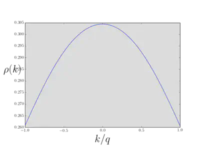
This is an integral equation that we must solve to find the ground state distribution of the \(\rho(k)\) in the thermodynamic limit, subject to the condition of fixed density \(n\)

\[ n\equiv \frac{N}{L} = \int_{-q}^q \rho(k)dk. \]

In terms of \(\rho(k)\), the momentum and energy are

\[ P_\text{tot} = L \int_{-q}^q k\rho(k)dk,\quad E_\text{tot} = L \int_{-q}^q \frac{k^2}{2}\rho(k)dk. \]

Of course, the momentum will vanish in the ground state, as \(\rho(k)\) will be an even function. If we fix the density \(n\), there is a natural dimensionless parameter \(\gamma\equiv c/n\), in terms of which we can express the energy per particle \(E_\text{tot}/L =\frac{n^3}{2}e(\gamma)\).

In the \(\gamma\to\infty\) limit we have \(\rho(k) = 1/(2\pi)\), \(q=k_\text{F}\), and \(n=k_\text{F}/\pi\), so that

\[ e(\gamma\to\infty) = \frac{2}{n^3}\int_{-q}^q \frac{k^2}{2}\rho(k)dk = \frac{1}{\pi n^3} \frac{k_\text{F}^3}{3} = \frac{\pi^2}{3} \]

Although I’ve referred to the \(k_j\) above as the momenta of the particles, this is actually highly misleading. In particular, the momentum distribution \(\bar N_k\) introduced in the previous lecture does not correspond to the distribution \(\rho(k)\) studied here. One way to convince yourself of this fact is to note that the second moment of \(\rho(k)\) gives the total energy, while the second moment of \(\bar N_k\) gives only the kinetic energy.

Finding \(\bar N_k\) is not straightforward for wavefunctions that are not product states of momentum eigenstates. For this reason it’s useful to refer to the \(k_j\) in the Bethe wavefunction as quasimomenta. Note that \(P_\text{tot}\) is, however, the true total momentum!

Excited States

Next we’d like to get a handle on the excited states. Again, we take our cue from the impenetrable limit, where we can think about the excitations of a Fermi gas. In this system, the basic excitation is the particle-hole pair, meaning that we take a particle from below the Fermi energy and move it above, leaving a hole behind.

In terms of the momenta \(k_\text{p}\), \(k_\text{h}\) of the particle and hole, the energy and momentum of such a state is

\[ \begin{align} E_\text{ph}(k_\text{p},k_\text{h}) &= \frac{1}{2}\left(k_\text{p}^2 - k_\text{h}^2\right),\qquad \abs{k_\text{p}}>k_\text{F}, \abs{k_\text{h}}<k_\text{F}\\ P_\text{ph}(k_\text{p},k_\text{h}) &= k_\text{p}-k_\text{h}. \end{align} \]

At fixed momentum, the highest (lowest) energy particle-hole pair has the hole (particle) at the Fermi surface. The extremal energies are

\[ \begin{align} \epsilon_I(P) = Pk_\text{F}+ P^2/2\\ \epsilon_{II}(P) = Pk_\text{F}- P^2/2. \end{align} \]

We can keep track of these excitations as we reduce \(c\) from \(\infty\). Lieb and Liniger christened them ‘type I’ and ‘type II’ excitations.

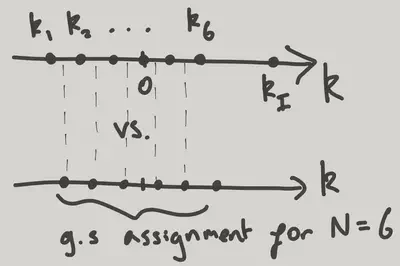
Let’s consider the type I excitations first. We imagine making a ‘hole’ in the distribution of roots and moving one particle above the ‘Fermi surface’ (by which I mean the largest root in the ground state distribution). The complication now is that doing so causes all the other roots to change slightly from their ground state values.

Instead of solving \(\eqref{LL_BE}\) with a set of consecutive integers on the right hand side, the final (largest) root – we’ll call it \(k_{I}\) – should correspond to an integer ‘standing apart’ from the others. We can think of this as the ground state of an \(N-1\) particle problem, with the \(N-1\) roots being affected by the presence of another root at \(k_{I}\). However, if we want to get the \(N\) particle ground state back as \(k_I\) returns to join the others, we have to choose an assignment of the \(I_j\) corresponding to \(N\) particles, not \(N-1\).

Let’s write the shift in the ground state roots of the \(N-1\) particle problem as \(\delta k_{i}\). Then we have

\[ \delta k_{i}L+\pi=\sum_{j=1}^{N-1}\theta'(k_{i}-k_{j})(\delta k_{i}-\delta k_{j})+\theta(k_{i}-k_{I}),\qquad i=1,2,\ldots, N-1. \]

The shifts \(\delta k_{i}\) are \(O(1/L)\). Taking \(\delta k\) to be a function of \(k\), we define the quantity \(\gamma(k)\equiv \delta k \rho(k)L\). Then it can be shown that \(\gamma(k)\) is a solution of

\[ -\int_{-q}^{q}\theta'(k-k')\gamma(k') dk'+\theta(k-k_{I})=\pi+2\pi \gamma(k),\qquad |k_{I}|>q. \label{LL_typeI} \]

To derive this equation we need the integral equation for \(\rho(k)\) \(\eqref{LL_BetheIntegral}\).

The energy and momentum of the excitation (that is, the energy and momentum difference of this state from the ground state) are

\[ \begin{align} \epsilon_{I}&=-\mu+\frac{k_{I}^{2}}{2}+\int_{-q}^{q}k\gamma(k)dk\nonumber\\ P&=k_{I}+\int_{-q}^{q}\gamma(k)dk \label{LL_disp} \end{align} \]

where \(\mu=E_{0}(N)-E_{0}(N-1)\) is the difference in ground state energies for \(N\) and \(N-1\) particles.

In these equations \(k_{I}\) is a parameter that determines \(\gamma(k)\) from \(\eqref{LL_typeI}\) and the dispersion relation \((E,P)\) is generated parametrically. Note that in \(\eqref{LL_disp}\) the last term in each expression is the result of the other roots being pushed around.

Now we turn to the type II excitations. By taking \(\delta k\) to be the shift in the roots of the ground state of the \(N+1\) particle problem caused by the presence of a hole, we can show that the corresponding set of equations is

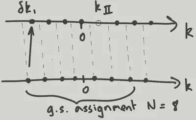
\[ \begin{align}\label{typeII} &-2\pi \gamma(k)+\pi-\int_{-q}^{q}\theta'(k-k')\gamma(k') dk'-\theta(k-k_{II})=0,\qquad |k_{II}|<q \nonumber\\ \epsilon_{II}&=\mu-\frac{k_{I}^{2}}{2}+\int_{-q}^{q}k\gamma(k)dk\nonumber\\ P&=-k_{II}+\int_{-q}^{q}\gamma(k)dk. \end{align} \]

References

{% bibliography –cited %}