\[ \nonumber \newcommand{\br}{\mathbf{r}} \newcommand{\bp}{\mathbf{p}} \newcommand{\bk}{\mathbf{k}} \newcommand{\bq}{\mathbf{q}} \newcommand{\bv}{\mathbf{v}} \newcommand{\pop}{\psi^{\vphantom{\dagger}}} \newcommand{\pdop}{\psi^\dagger} \newcommand{\Pop}{\Psi^{\vphantom{\dagger}}} \newcommand{\Pdop}{\Psi^\dagger} \newcommand{\Phop}{\Phi^{\vphantom{\dagger}}} \newcommand{\Phdop}{\Phi^\dagger} \newcommand{\phop}{\phi^{\vphantom{\dagger}}} \newcommand{\phdop}{\phi^\dagger} \newcommand{\aop}{a^{\vphantom{\dagger}}} \newcommand{\adop}{a^\dagger} \newcommand{\bop}{b^{\vphantom{\dagger}}} \newcommand{\bdop}{b^\dagger} \newcommand{\cop}{c^{\vphantom{\dagger}}} \newcommand{\cdop}{c^\dagger} \newcommand{\bra}[1]{\langle{#1}\rvert} \newcommand{\ket}[1]{\lvert{#1}\rangle} \newcommand{\inner}[2]{\langle{#1}\rvert #2 \rangle} \newcommand{\braket}[3]{\langle{#1}\rvert #2 \lvert #3 \rangle} \newcommand{\sgn}{\mathrm{sgn}} \DeclareMathOperator{\tr}{tr} \DeclareMathOperator{\E}{\mathbb{E}} \]
We begin our study of many body quantum mechanics by examining a number of systems where eigenstates and eigenvalues may be found explicitly for any number of particles. Be warned that these situations are highly atypical – but are nevertheless very informative.
Reading: {% cite Baym:1969 %}.
Bosons and Fermions
An \(N\) particle quantum system is described by a wavefunction of \(N\) arguments \(\Psi(\br_1,\ldots, \br_N)\). The starting point of many body quantum mechanics is that:
Systems of indistinguishable particles are described by totally symmetric or totally antisymmetric wavefunctions.
Just to be clear, totally symmetric means the wavefunction is unchanged by exchanging any two coordinates, whereas totally antisymmetric means that it changes sign.
A good fraction of this course is devoted to exploring the ramifications of this fact. Perhaps we should therefore give a very quick summary of why it appears to be true.
The first question is: what are indistinguishable particles? I’ll give a theorist’s answer. Indistinguishable particles are those described by Hamiltonians that are invariant under permuting the particle’s labels. Thus the sum of single particle Hamiltonians
\[ H = \sum_{i=1}^{N} \left[-\frac{\nabla_i^{2}}{2m}+V(\mathbf{r_i})\right] \]
[did you remember that \(\hbar=1\)?] describes indistinguishable particles while
\[ H = \sum_{i=1}^{N} \left[-\frac{\nabla_i^{2}}{2m_i}+V(\mathbf{r_i})\right] \]
does not, on account of the masses being all different. Any time we have a symmetry operation that commutes with the Hamiltonian, the eigenstates of that symmetry are preserved by time evolution with that Hamiltonian. Thus a symmetric potential \(V(x)=V(-x)\) commutes with the parity operation \(x\to -x\), so the eigenstates of this operation – the even and odd wavefunctions – are preserved by time evolution.
The Hamiltonian of indistinguishable particles commutes with every operator of particle exchange, defined by \[ P_{ij}\Psi(\br_1,\ldots, \br_i,\ldots, \br_j,\ldots \br_N) = \Psi(\br_1,\ldots, \br_j,\ldots, \br_i,\ldots \br_N). \]
These operators satisfy \(P_{ij}^2=\mathbb{1}\), so their eigenvalues are \(\pm 1\), corresponding to states that are either symmetric or antisymmetric under exchange. The only simultaneous eigenstates of all particle exchange operations (note that different exchanges don’t commute if they involve the same particle) are the totally symmetric and antisymmetric wavefunctions. Thus these properties are preserved by time evolution. It’s always been this way.
We classify particles into symmetric bosons and antisymmetric fermions, named for Bose and Fermi respectively (the whimsical terminology is Dirac’s). The distinction works equally well for composite particles, provide we ignore the internal degrees of freedom and discuss only the center of mass coordinate.
All matter in the universe is made up of fermions: electrons, quarks, etc., but you can easily convince yourself that an even number of fermions make a composite boson (e.g. a \(^4\)He atom with two electrons, two neutrons and two protons) and an odd number make a composite fermion (\(^3\)He has one fewer neutron, which in turn is made up of 3 quarks).
Two Particles
A pair of particles is described by a wavefunction \(\Psi(\mathbf{x},\mathbf{y})\). If we are dealing with distinguishable particles, the wavefunction of a pair of particles in states \(\ket{\varphi_1}\) and \(\ket{\varphi_2}\) would be
\[ \Psi(\br_1,\br_2)=\varphi_1(\br_1)\varphi_2(\br_2). \label{quantum_statistics_ProductWavefunction} \]
Accounting for indistinguishability, we have either
\[ \label{quantum_statistics_sym} \Psi(\br_1,\br_2)=\frac{1}{\sqrt{2}}[\varphi_1(\br_1)\varphi_2(\br_2)\pm \varphi_2(\br_1)\varphi_1(\br_2)] \]
with the upper sign for bosons and the lower for fermions (The \(1/\sqrt{2}\) yields a normalized wavefunction if \(\varphi_{1,2}(\br)\) are orthonormal.). Note in particular that when \(\varphi_1=\varphi_2\) the fermion wavefunction vanishes. This illustrates the Pauli exclusion principle, that no two identical fermions can be in the same quantum state. There is no such restriction for bosons.
Classically, if you had a function \(\rho_{1}(\br_1)\) describing the probability density of finding particle \(1\) at position \(\br_1\), and the corresponding quantity for an independent particle \(2\), you would have no hesitation in concluding that the joint distribution is
\[ \rho_{12}(\br_1,\br_2)=\rho_1(\br_1)\rho_2(\br_2). \label{eq:classicaljoint} \]
This also follows from taking the square modulus of \(\eqref{quantum_statistics_ProductWavefunction}\). The result implied by the wavefunction \(\eqref{quantum_statistics_sym}\) is \[ \begin{align} \rho_{12}(\br_1,\br_2) &= \frac{1}{2}\left[\rho_1(\br_1)\rho_2(\br_2)+\rho_1(\br_2)\rho_2(\br_1)\right] \\ &\pm\frac{1}{2}\left[\varphi^{}_1(\br_1)\varphi^*_2(\br_1)\varphi^{}_2(\br_2)\varphi^*_1(\br_2)+\varphi^{}_1(\br_2)\varphi^*_2(\br_2)\varphi^{}_2(\br_1)\varphi^*_1(\br_1)\right]. \end{align} \]
In particular, \(\rho_{12}(\br,\br) = 0\) for fermions, and \(\rho_{12}(\br,\br) = 2\rho_1(\br)\rho_2(\br)\) for bosons. The first result is natural from the standpoint of the exclusion principle, while the second is perhaps more surprising. This shows that, because probabilities arise from the squares of amplitudes, identical particles in quantum mechanics are never truly independent.
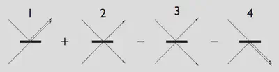
One dramatic illustration of this deviation from our classical intuition is provided by the Hong–Ou–Mandel effect in quantum optics. In simplified terms, we imagine wavepackets describing two photons (bosons) approaching a 50:50 beam splitter from either side. Because of the unitarity of scattering, the two photons end up in orthogonal states. For example, \[ \begin{align} \ket{\text{Left}}\to\frac{1}{\sqrt{2}}\left(\ket{\text{Left}}+ \ket{\text{Right}}\right)\\\\ \ket{\text{Right}}\to\frac{1}{\sqrt{2}}\left(\ket{\text{Left}}- \ket{\text{Right}}\right) \end{align} \]
If we start in \[ \frac{1}{\sqrt{2}}[\varphi_\text{L}(\br_1)\varphi_\text{R}(\br_2)\pm \varphi_\text{R}(\br_1)\varphi_\text{L}(\br_2)] \] What state do we end up in?
Product States
The Hamiltonian of a system of \(N\) identical noninteracting particles is a sum of \(N\) identical single particle Hamiltonians, that is, with each term acting on a different particle coordinate
\[ H = \sum_{i=1}^{N} \left[-\frac{\nabla_i^{2}}{2m}+V(\br_i)\right] \label{quantum_statistics_SPHamiltonian} \]
where \(m\) is the particle mass, and \(V(\br)\) is a potential experienced by the particles.
Let’s denote the eigenstates of the single particle Hamiltonian by \(\{\varphi_\alpha(\br)\}\) , and the corresponding eigenenergies by \(\{E_\alpha\}\), where \(\alpha\) is a shorthand for whatever quantum numbers are used to label the states.
A set of labels \(\{\alpha_{i}\}\) \(i=1,2,\ldots N\) tells us the state of each of the particles. Thus we can write an eigenstatof \(N\) distinguishable particles with energy \(E=\sum_{i=1}^{N}E_{\alpha_{i}}\) as
\[ \label{quantum_statistics_disting} \ket{\Psi_{\alpha_{1}\alpha_{2}\cdots \alpha_{N}}}=\varphi_{\alpha_{1}}(\mathbf{r_{1}})\varphi_{\alpha_{2}}(\mathbf{r_{2}})\cdots\varphi_{\alpha_{N}}(\mathbf{r_{N}}) \]
(We will frequently switch between the wavefunction \(\varphi(\mathbf{x})\) and bra-ket notation \(\ket{\varphi}\). In the latter notation the product wavefunction in \(\eqref{quantum_statistics_ProductWavefunction}\) is written \(\ket{\varphi_{1}}\ket{\varphi_{2}}\))
Such states are called product states. A general state will be expressed as a superposition of product states: they are special states which provide a frequently convenient basis.
As we’ve just discussed, however, we should really be dealing with a totally symmetric or totally antisymmetric wavefunction, depending on whether our identical particles are bosons or fermions. To write these down we introduce the operators of symmetrization and antisymmetrization
\[ \label{quantum_statistics_SymAntisym} \mathcal{S}=\frac{1}{N!}\sum_{\pi} P_\pi, \qquad \mathcal{A}=\frac{1}{N!}\sum_{\pi} \sgn(\pi)P_\pi \]
Here’s the definition of the various quantities in \(\eqref{quantum_statistics_SymAntisym}\):
- The sums are over all \(N!\) permutations \(\pi\) of \(N\) objects. One way to think of a permutation \(\pi\) is as a one-to-one correspondence (or bijection) between the set \(\{1,2,\ldots N\}\) and itself, so that 1 is mapped to \(\pi(1)\), etc..
- \(P_\pi\) denotes the corresponding permutation operator \[ P_\pi \Psi(\br_1,\br_2,\ldots \br_N) = \Psi(\br_{\pi(1)}, \br_{\pi(2)},\ldots \br_{\pi(N)}) \]
- \(\sgn(\pi)\) is the signature of the permutation, equal to \(+1\) for permutations involving an even number of exchanges, and \(-1\) for an odd number.
\(\eqref{quantum_statistics_SymAntisym}\) allows us to write the totally symmetric and totally antisymmetric versions of \(\eqref{quantum_statistics_disting}\) as \[ \begin{align} \ket{\Psi^{S}_{\alpha_{1}\alpha_{2}\cdots\alpha_{N}}}&=\sqrt{N!\prod_{\alpha}N_{\alpha}!}\mathcal{S}\,\varphi_{\alpha_{1}}(\mathbf{r_{1}})\varphi_{\alpha_{2}}(\mathbf{r_{2}})\cdots\varphi_{\alpha_{N}}(\mathbf{r_{N}}) \nonumber \\ \ket{\Psi^{A}_{\alpha_{1}\alpha_{2}\cdots\alpha_{N}}}&=\sqrt{N!}\mathcal{A}\,\varphi_{\alpha_{1}}(\mathbf{r_{1}})\varphi_{\alpha_{2}}(\mathbf{r_{2}})\cdots\varphi_{\alpha_{N}}(\mathbf{r_{N}}) \label{quantum_statistics_norm} \end{align} \]
The normalization factors yield normalized wavefunctions if the single particle state \(\ket{\varphi_\alpha}\) are orthonormal (as the eigenstates of the single particle Hamiltonian are).
The normalization factor in the boson case involves the occupation numbers \(\{N_{\alpha}\}\) giving the number of particles in state \(\alpha\). In the fermion case each \(N_{\alpha}\) is either \(0\) or \(1\) so the prefactor simplifies. Since the order of the \(\alpha\) indices is irrelevant in the boson case, and amounts only to a sign in the fermion case, states based on a given set of single particle states are more efficiently labeled by the occupation numbers. In terms of these numbers the total energy is
\[ \label{quantum_statistics_TotalEnergy} E=\sum_{i=1}^{N}E_{\alpha_{i}}=\sum_{\alpha}N_{\alpha} E_{\alpha} \]
Verify that the normalization factors in \(\eqref{quantum_statistics_norm}\) are correct.
A more formal way of putting things is as follows. We first consider the space spanned by states of the form \(\eqref{quantum_statistics_disting}\). Then we introduce the operators \(\mathcal{S}\) and \(\mathcal{A}\), noting that \(\mathcal{S}^{2}=\mathcal{S}\) and \(\mathcal{A}^{2}=\mathcal{A}\). In other words, there’s no point symmetrizing or antisymmetrizing more than once (we say that the operators are idempotent). Any eigenvalue of one of these operators is therefore either one or zero. The states with \(\mathcal{S}=1\) are the symmetric states, and those with \(\mathcal{A}=1\) are antisymmetric. You can easily convince yourself that if a state has one of \(\mathcal{S}\) or \(\mathcal{A}\) equal to one, the other is zero. This defines symmetric and antisymmetric subspaces, consisting of the admissible boson and fermion wavefunctions.
Note that the fermion wavefunction takes the form of a Slater determinant (though it appears first in {% cite dirac1926 %}).
\[ \label{quantum_statistics_slater} \ket{\Psi^{A}_{\alpha_{1}\alpha_{2}\cdots\alpha_{N}}}=\frac{1}{\sqrt{N!}}\begin{vmatrix} \varphi_{\alpha_{1}}(\mathbf{r_{1}}) & \varphi_{\alpha_{1}}(\mathbf{r_{2}}) & \cdots & \varphi_{\alpha_{1}}(\mathbf{r_{N}}) \\ \varphi_{\alpha_{2}}(\mathbf{r_{1}}) & \cdots & \cdots & \cdots \\ \cdots & \cdots & \cdots & \cdots \\ \varphi_{\alpha_{N}}(\mathbf{r_{1}}) & \cdots & \cdots & \varphi_{\alpha_{N}}(\mathbf{r_{N}}) \end{vmatrix} \]
The vanishing of a determinant when two rows or two columns are identical means that the wavefunction is zero if two particle coordinates coincide (\(\br_{i}=\br_{j}\)), or if two particles occupy the same state (\(\alpha_{i}=\alpha_{j}\)).
The 1D Fermi Gas
Let’s consider perhaps the simplest many particle system one can think of: noninteracting particles on a ring. If the ring has circumference \(L\), the single particle eigenstates are \[ \label{quantum_statistics_spstates} \varphi_{n}(x)=\frac{1}{\sqrt{L}}\exp\left(ik_n x\right), \]
with \(k_n=\frac{2\pi n}{L}\), \(n\in\mathbb{Z}\). The corresponding energies are \(E_{n}=\frac{k_n^2}{2m}\).
Ground State
Let’s find the \(N\) particle ground state. For bosons every particle is in the state \(\ket{\varphi_{0}}\) with zero energy: \(N_{0}=N\). Thus
\[ \Psi^{S}(x_{1},x_{2},\ldots x_{N})=\frac{1}{L^{N/2}} \]
That was easy! The fermion case is harder.
Since the occupation of each level is at most one, the lowest energy is obtained by filling each level with one particle, starting at the bottom. If we have an odd number of particles, this means filling the levels with \(n=-(N-1)/2, -(N-3)/2,\ldots, -1, 0, 1 \ldots (N-1)/2\) (for an even number of particles we have to decide whether to put the last particle at \(n=\pm N/2\)). Introducing the complex variables
\[ z_{i}=\exp(2 \pi i x_{i}/L), \]
the Slater determinant \(\eqref{quantum_statistics_slater}\) becomes
\[ \label{quantum_statistics_1ddet} \Psi_0(x_1,\ldots, x_N)=\begin{vmatrix} z_{1}^{-(N-1)/2} & z_{2}^{-(N-1)/2} & \cdots & z_{N}^{-(N-1)/2} \\ z_{1}^{-(N-3)/2} & \cdots & \cdots & \cdots \\ \cdots & \cdots & \cdots & \cdots \\ z_{1}^{(N-1)/2} & \cdots & \cdots & z_{N}^{(N-1)/2} \end{vmatrix}. \]
Let’s evaluate this complicated looking expression in a simple case. With three particles we have
\[ \begin{align} \Psi_0(x_1,x_2,x_3)&=\begin{vmatrix} z_{1}^{-1} & z_{2}^{-1} & z_{3}^{-1} \\ 1 & 1 & 1 \\ z_{1} & z_{2} & z_{3} \end{vmatrix} = \frac{z_{1}}{z_{2}}-\frac{z_{2}}{z_{1}}+\frac{z_{3}}{z_{1}}-\frac{z_{1}}{z_{3}}+\frac{z_{2}}{z_{3}}-\frac{z_{3}}{z_{2}}\nonumber\\ &=\left(\sqrt{\frac{z_{3}}{z_{1}}}-\sqrt{\frac{z_{1}}{z_{3}}}\right)\left(\sqrt{\frac{z_{1}}{z_{2}}}-\sqrt{\frac{z_{2}}{z_{1}}}\right)\left(\sqrt{\frac{z_{2}}{z_{3}}}-\sqrt{\frac{z_{3}}{z_{2}}}\right) \nonumber\\ &\propto \sin\left(\frac{ \pi[x_{1}-x_{2}]}{L}\right)\sin\left(\frac{ \pi[x_{3}-x_{1}]}{L}\right)\sin\left(\frac{ \pi[x_{2}-x_{3}]}{L}\right) \label{3particle} \end{align} \]
The vanishing of the wavefunction when \(x_{i}=x_{j}\) is consistent with the Pauli principle. You should check that additionally it is periodic and totally antisymmetric.
\(\eqref{3particle}\) generalizes for any (odd) \(N\) so that the ground state Slater determinant \(\eqref{quantum_statistics_1ddet}\) is proportional to
\[ \Psi_0(x_1,\ldots, x_N)\propto\prod_{i<j}^{N} \sin\left(\frac{\pi[x_{i}-x_{j}]}{L}\right). \label{quantum_statistics_1dFermiGS} \]
Show this using the Vandermonde determinant \[ \begin{vmatrix} 1 & 1 & \cdots & 1 \\ z_{1} & z_{2} & \cdots & \cdots \\ z_{1}^{2} & z_{2}^{2} & \cdots & \cdots \\ z_{1}^{N-1} & z_{2}^{N-1} & \cdots & z_{N}^{N-1} \end{vmatrix}=\prod_{i<j}^{N}(z_{j}-z_{i}) \] which can be proved in a variety of ways. Proving directly that \(\eqref{quantum_statistics_1dFermiGS}\) is an eigenstate of the Hamiltonian is not easy, but can be accomplished using the identity
\[ \begin{equation} \label{2nd_quant_cotident} \cot(x-y)\cot(y-z)+\cot(y-z)\cot(z-x)+\cot(z-x)\cot(x-y)=1. \nonumber \end{equation} \]
Check carefully that \(\eqref{quantum_statistics_1dFermiGS}\) is periodic and totally antisymmetric.
Let’s take the opportunity to introduce some terminology. The wavevector of the last fermion added is called the Fermi wavevector and denoted \(k_\text{F}\). In this case \(k_\text{F}=\frac{(N-1)\pi}{L}\). Its energy \(E_{F}=\frac{k_\text{F}^{2}}{2m}\) is the Fermi energy.
Density; Density Matrix; Pair Distribution
Having a many particle wave function is one thing, but what to do with it? Bear in mind that \(\eqref{quantum_statistics_1dFermiGS}\) is just about the simplest fermion state you can imagine, but it’s not immediately clear what it is telling us.
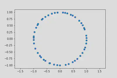
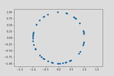
\(\vert\Psi(x_1,\ldots,x_N)\rvert^2\) is the probability distribution of the positions of the particles. If we were able to take a photograph of the positions of the particles at an instant in time, this would correspond to taking a sample from the probability distribution. In terms of the complex variables \(z_j\), it would look something like this:
Since \(\lvert\Psi(x_1,\ldots,x_N)\rvert^2\) is the probability distribution of the positions of the particles, we can use it to find the marginal probability distributions for any subset of the particles. Of course, since the particles are identical, it doesn’t matter which ones we choose, just the number.
The one particle distribution is related to the average density of particles, given by \[ \rho_1(x_1) = N \int dx_2\ldots dx_N \,\lvert\Psi(x_1,x_2,\ldots,x_N)\rvert^2. \label{ave_density} \] Note that although I use the symbol \(\rho\), density is always going to be number density (not the mass density).
Can you explain why this is the density? Think about the simpler case of two particles, with discrete locations. Why is the expected number of particles at position \(x\)
\[ N_x = \sum_y \left[P(x,y) + P(y,x)\right]? \]
What if we have more particles?
Normalization of the wavefunction then implies \[ \int dx\, \rho_1(x) = N. \] In a translationally invariant system like the fermion gas on a ring we expect the average density to be constant.
We can regard \(\eqref{ave_density}\) as an expectation of a density operator \[ \rho(x) = \sum_j \delta(x-x_j), \label{many_densityop} \] so that \(\rho_1(x) = \braket{\Psi}{\rho(x)}{\Psi}\).
The single particle density matrix is a generalization of the expectation of the density, and is defined as (we’ll see shortly why this is a useful quantity) \[ \label{eq:spdm} g(x,y) \equiv N\int dx_2\ldots dx_N \,\Psi^{}(x,x_2,\ldots,x_N)\Psi^{*}(y,x_2,\ldots,x_N). \] Note that \(g(x,x) = \rho_1(x)\).
Show that the average number of particles in a single particle state \(\ket{\psi}\) is \[ \bar N_\psi = \int dx dy\, \psi^*(x)g(x,y)\psi(y). \label{many_Nbar} \]
Starting from the Slater determinant \(\eqref{quantum_statistics_1ddet}\) (i.e. not from the explicit form \(\eqref{quantum_statistics_1dFermiGS}\)), show that \(g(x,y)\) for the ground state of the Fermi gas is \[ g(x,y) = \frac{1}{L}\sum_{|k|<k_\text{F}} e^{ik(x-y)} = \int_{k_\text{F}}^{k_\text{F}} \frac{dk}{2\pi} e^{ik(x-y)} = n \frac{\sin \left[k_\text{F}(x-y)\right]}{k_\text{F}(x-y)} \] where \(n \equiv \frac{k_\text{F}}{\pi}\) is the average density.
Find the average number of particles in a momentum state \(\ket{k}\) using \(\eqref{many_Nbar}\) \[ \bar N_k = \begin{cases} 1 & |k|\leq k_\text{F} \\ 0 & |k|>k_\text{F} \end{cases}. \label{many_Nk} \] Note that in a translationally invariant system \(g(x,y)=g(x-y)\), and is the Fourier transform of \(\bar N_k\).
To understand the origin of the name single particle density matrix, recall that the density matrix \(\varrho\) describes a mixed state of a quantum system, and is the appropriate description when the quantum state is not known. \(\varrho\) is a positive definite hermitian operator satisfying \(\tr \varrho =1\). Its spectral resolution \[ \varrho = \sum_\alpha p_\alpha \ket{\varphi_\alpha}\bra{\varphi_\alpha}, \] can be thought of as a statistical mixture of different quantum states \(\ket{\varphi_\alpha}\) with probabilities \(p_\alpha\).
One natural way in which density matrices arise from pure states is as follows. The Hilbert space of a composite system consists of a tensor product of two or more components \(\mathcal{H}_{AB} = \mathcal{H}_A \otimes \mathcal{H}_B\). Starting from the density matrix corresponding to a pure state, we can obtain a density matrix for the component \(A\) alone by ‘tracing out’ the \(B\) subsystem. \[ \varrho_A = \tr_B \ket{\Psi}\bra{\Psi},\quad \ket{\Psi}\in \mathcal{H}_{AB}. \] The probability for system \(A\) to be in state \(\ket{\psi}\in \mathcal{H}_A\) is \[ P_\psi = \bra{\psi}\varrho\ket{\psi}. \] Thus you can think of the single particle density matrix as arising from tracing out \(N-1\) particles from an \(N\)-particle system.
We can also consider marginal probability distribution of a pair of particles, and define the pair distribution function \[ \rho_2(x_1,x_2) = N(N-1) \int dx_3\ldots dx_N \,\left|\Psi(x_1,x_2,\ldots,x_N)\right|^2. \] The prefactor is to account for all pairs of particles.
Starting from the Slater determinant \(\eqref{quantum_statistics_1ddet}\), show that \[ \rho_2(x_1,x_2) = n^2\left[1 - \left(\frac{\sin\left[k_\text{F}(x_1-x_2)\right]}{k_\text{F}(x_1-x_2)}\right)^2\right]. \] This vanishes at \(x_1=x_2\), consistent with the Pauli principle.
A natural question: \[ \rho_2(x_1,x_2) \overset{?}{=} \bra{\Psi}\rho(x_1)\rho(x_2)\ket{\Psi}. \] Almost. Looking back at \(\eqref{many_densityop}\), we see that the product of two density operators will contain terms involving the same particle, which are absent from \(\rho_2(x_1,x_2)\).
Show that the correct relationship is \[ \rho_2(x_1,x_2) = \bra{\Psi}\rho(x_1)\rho(x_2)\ket{\Psi} - \rho_1(x_1)\delta(x_1-x_2). \]
Impenetrable Bose Gas
There’s a bit more mileage in the 1D Fermi gas yet. Consider the following Hamiltonian, which we’ll study in more detail in Lecture 15 \[ H = -\frac{1}{2m}\sum_j \frac{\partial^2}{\partial x_j^2} + \overbrace{c\sum_{j<k}\delta(x_j-x_k)}^{\equiv H_\text{int}}. \label{many_LL} \] The second term represents an interaction between pairs of particles. Of course, this model is rather special, as (1) it’s 1D and (2) the interaction potential is a \(\delta\)-function. Nevertheless, it represents a huge step up in difficulty from the noninteracting examples we’ve discussed so far. At least, it does for bosons. For fermions, the wavefunctions vanish at coincident points, and so the interaction has no effect at all!
For bosons, it happens that the Hamiltonian can still be solved exactly. For now, however, we’ll concern ourselves only with the limit of infinite interaction: \(c\to \infty\), sometimes called the impenetrable limit. In this case, the eigenenergies coincide with those of the free fermion problem, and the eigenstates are just the modulus of the corresponding fermion eigenstate.
Why?
Just like that, we’ve solved our first interacting many body system (and with infinite coupling, no less)!
Thus the ground state on the ring has the form \[ \Psi_0(x_1,\ldots, x_N) = \prod_{i<j}^{N} \left|\sin\left(\frac{\pi[x_{i}-x_{j}]}{L}\right)\right|. \]
It’s not hard to see why this works. For a state to have a finite energy, the wavefunction must vanish whenever two coordinates coincide. This is because the interation energy has the expectation value \[ \braket{\Psi}{H_\text{int}}{\Psi}=cN(N-1)\int dx_1\cdots dx_{N-1}\left| \Psi(x_1,x_1,x_2,\ldots,x_N\right|^2 \] But we already have a complete set of eigenstates that obey this condition, namely the free fermion Slater determinants. It remains to make them symmetric functions by taking the modulus.
This mapping is quite powerful, and allows us to calculate any observable of the impenetrable Bose gas in terms of free fermions as long as that observable is insensitive to taking the modulus of the wavefunction. Thus the average density \(\rho_1(x)\) and pair distribution \(\rho_2(x_1,x_2)\) of the previous section can be found in this way, but the single particle density matrix \(g(x,y)\) cannot.
Show this explicitly.
This means that the momentum distribution is not given by \(\eqref{many_Nk}\). Finding \(g(x,y)\) for the impenetrable Bose gas is in fact really hard. We’ll see in a later lecture how to obtain some of its important features.
References
{% bibliography –cited %}