Bose Gas

Noninteracting bosons form a Bose–Einstein condensate (BEC)
What do interactions do?
BEC closely related to superfluidity

Gross–Pitaevskii Approximation

Variational appraoch to Bose gas (c.f. Hartree–Fock)
Put all particles in same single particle state!

$$ \Psi(\br_1,\ldots \br_N) = \prod_{j=1}^N \varphi_0(\br_i)= \frac{1}{\sqrt{N!}}\left(\adop(\varphi_0)\right)^N\ket{\text{VAC}}. $$

State with macroscopic number of particles in a single particle state is a Bose condensate

For noninteracting Hamiltonian

$$ H = \sum\left[-\frac{\nabla_i^2}{2m} + V(\br_i)\right], $$

Ground state is exactly $$ \Psi(\br_1,\ldots \br_N) = \prod_{j=1}^N \varphi_0(\br_i)= \frac{1}{\sqrt{N!}}\left(\adop(\varphi_0)\right)^N\ket{\text{VAC}}. $$ with $\varphi_0(\br)$ the ground state of single particle Hamiltonian

Add interaction

$$ \begin{align*} H_\text{int.} &= \sum_{j<k} U(\br_j-\br_k) \\ &= \frac{1}{2}\int d\br_1 d\br_2\, U(\br_1-\br_2)\pdop(\br_1)\pdop(\br_2)\pop(\br_2)\pop(\br_1) \end{align*} $$

Ground state is more complicated, but can use BEC form with $\varphi_0(\br)$ as a variational function
Optimal $\varphi_0(\br)$ obeys Gross–Pitaevskii equation

Gross–Pitaevskii Equation

Take short-ranged interactions for simplicity

$$ U(\br-\br’) = U_0\delta(\br-\br’) $$

For variational calculation we need

$$ \langle E \rangle = \frac{\braket{\Psi|H|\Psi}}{\braket{\Psi|\Psi}} $$

Minimize $\braket{\Psi|H|\Psi}$ and fix norm. using Lagrange multiplier

$$ \begin{align*} \braket{\Psi|H|\Psi}=N \int d\br \left[\frac{1}{2m}|\nabla\varphi_0|^2+V(\br)|\varphi_0(\br)|^2 \right]\\ +\frac{1}{2}N(N-1)U_0\int d\br |\varphi_0(\br)|^4 \end{align*} $$

Neglect difference between $N$ and $N+1$ $$ \begin{align*} \braket{\Psi|H|\Psi}=N \int d\br \left[\frac{1}{2m}|\nabla\varphi_0|^2+V(\br)|\varphi_0(\br)|^2 \right]\\ +\frac{1}{2}N^2 U_0\int d\br |\varphi_0(\br)|^4 \end{align*} $$
Extremize the functional

$$ \braket{\Psi|H|\Psi} - \mu N \int d\br |\varphi_{0}(\br)|^{2}. $$

Calculus of variations yields

$$ \left[-\frac{1}{2m}\nabla^2-\mu+V(\br)+NU_0|\varphi_0(\br)|^2\right]\varphi_0(\br)=0 $$

Define $\varphi(\br)\equiv\sqrt{N}\varphi_{0}(\br)$
$\varphi(\br)$ is condensate wavefunction or order parameter. Obeys Gross–Pitaevskii equation

$$ \left[-\frac{1}{2m}\nabla^2-\mu+V(\br)+U_0|\varphi(\br)|^2\right]\varphi(\br)=0. $$

Fix Lagrange multiplier $\mu$ by $\int d\br\abs{\varphi(\br)}^{2}=N$
$\braket{\Psi|H|\Psi}- \mu \int d\br \abs{\varphi(\br)}^{2}=\braket{\Psi|H-\mu \mathsf{N}|\Psi}$ was extremized under general variations, including change in $N$ $$ \mu=\frac{\partial\braket{\Psi|H|\Psi}}{\partial N}, $$ $\mu$ is identified with the chemical potential.

Healing length

1D, no potential

$$ \left[-\frac{1}{2m}\partial_x^2-\mu+U_0|\varphi|^2\right]\varphi(x)=0. $$

Dimensionless form $\varphi(\br)=\sqrt{n}\phi(\br/\xi)$ for $\mu=U_0n$

$$ -\frac{1}{2m \xi^2}\phi''+\mu (|\phi|^2-1)\phi(x)=0. $$

If we set $\xi\equiv \frac{1}{\sqrt{2m \mu}}=\frac{1}{\sqrt{2m n U_0}}$ then

$$ -\phi''+(|\phi|^2-1)\phi(x)=0. $$

Healing length $\xi$ is scale on which $\varphi(\br)$ disturbed by localized perturbation of scale $\ll \xi$

Near a wall
$$ \varphi(x)=\varphi_{\infty}\tanh \frac{x}{\sqrt{2}\xi} $$
where $x$ is distance from wall, and $\varphi_{\infty}=\sqrt{n}$ is fixed by the density far away.

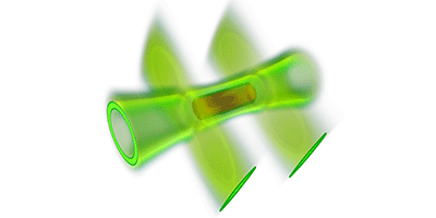
Condensate in a Can

drawing

Some Observables

Density and current density

$$ \begin{align*} \rho(\br)&=|\varphi(\br)|^2,\\ \mathbf{j}(\br)&=-\frac{i}{2m}\left[\varphi^{*}(\br)\left(\nabla\varphi(\br)\right)-\left(\nabla\varphi^{*}(\br)\right)\varphi(\br)\right] \end{align*} $$

Useful decomposition into magnitude and phase

$$ \varphi(\br)=\sqrt{\rho(\br)}e^{i\chi(\br)}. $$

Using $\mathbf{j}=\rho \mathbf{v}$ we get superfluid velocity

$$ \mathbf{v}_{s}\equiv\frac{1}{m}\nabla\chi. $$

Example: Vortex

Expect $\mathbf{v}_{s}=\frac{1}{m}\nabla\chi$ to be irrotational $$ \nabla\times \mathbf{v}_s = 0, $$
Equivalently to have vanishing circulation around any closed loop

$$ \oint \mathbf{v}_s\cdot d\mathbf{l}=0 $$

Phase can increase by a multiple of $2\pi$ around a closed loop, so $$ \oint \mathbf{v}_s\cdot d\mathbf{l}=\frac{2\pi \ell}{m},\quad \ell\in\mathbb{Z}, $$ Onsager–Feynmann quantization condition.

Localized configuration with finite circulation is a vortex in fluid dynamics
In normal fluid there is no reason for the vorticity to be quantized $$ \oint \mathbf{v}_s\cdot d\mathbf{l}=\frac{h\ell}{m},\quad \ell\in\mathbb{Z}, $$ shows that this is a truly quantum phenomenon.
A non-zero winding of phase requires that $\rho(\br)$ vanishes at a point (in 2D) or on a line (in 3D)

Look for 2D solutions where phase winds $\ell$ times around origin

$$ \varphi(r,\theta)\xrightarrow{r\to\infty} \sqrt{n} e^{i\ell\theta} $$

Paremeterize $\varphi(r,\theta) = \sqrt{n} f(r/\xi)e^{i\ell\theta}$ to give an equation in $s\equiv r/\xi$ (set $\mu=U_0 n$ as before).

$$ -f'' -\frac{f'}{s} + \frac{\ell^2 f}{s^2} - f +f^3 =0. $$

Without finding the solution explicitly, show that $f(s)\sim s^\ell$ for small $s$, and $f(s\to\infty) \to 1$.

Region of suppressed density size $\xi$, is vortex core
In three dimensions, vortex core is a line
Find energy of vortex by substituting solution back into energy

$$ \begin{align*} \braket{\Psi|H|\Psi}=\int d\br \left[\frac{1}{2m}|\nabla\varphi|^2+V(\br)|\varphi(\br)|^2 \right]+\frac{1}{2}U_0\int d\br |\varphi(\br)|^4. \end{align*} $$

Excess energy (relative to uniform state of density $n$)

$$ \Delta E = \int d\br \left[\frac{n^2}{2m\xi^2}(f')^2+\frac{U}{2}n^2 \left(f^2-1\right)^2\right] + \frac{n^2}{2m}\int d\br\, f^2(\nabla\chi)^2 $$

First integral is finite: due to density $\neq$ bulk value
Second is KE contribution from winding of vortex

$$ \nabla \chi = \frac{\ell}{r}\hat{\mathbf{e}}_\theta, $$

This contribution to the energy is logarithmically divergent.

$$ \Delta E = \text{const.} + \frac{\pi n \ell^2}{m}\log\left(\frac{L}{\xi}\right). $$

Far-reaching analogy between superfluid velocity fields of vortices and magnetostatics of current-carrying wires,

Vortices	Magnetostatics
Vortex cores	Wires
Superfluid velocity $\mathbf{v}_s$	Magnetic field, $\mathbf{B}$
Kinetic Energy	Magnetostatic Energy

Vortices with $\abs{\ell}>1$ generally unstable: break into multiple vortices of winding $\ell=\pm 1$

Like vortices repel each other, and can form spectacular vortex lattices, akin to crystals.

drawing

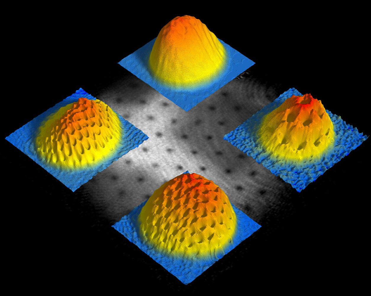
Vortices are one manifestation of superfluidity

Bogoliubov Theory

How can we improve Gross–Pitaevskii approximation?
What about excited states?
From now on… uniform condensate with no $V(\br)=0$

$$ H =\sum_\bk \epsilon(\bk)\adop_\bk\aop_\bk + \overbrace{\frac{U_0}{2V}\sum_{\bk_1+\bk_2=\bk_3+\bk_4} \adop_{\bk_1}\adop_{\bk_2}\aop_{\bk_3}\aop_{\bk_4}}^{\equiv H_\text{int}}, $$

$\epsilon(\bk)=\bk^2/2m$, and $V$ the volume
GP approximation to ground state is $\ket{\Psi_\text{GP}} = \frac{1}{\sqrt{N!}}\left(\adop_0\right)^N\ket{\text{VAC}}$
Act with $H_\text{int}$: only terms that contribute have $\bk_3=\bk_4=0$

$$ H_\text{int}\ket{\Psi_\text{GP}} = \frac{U_0}{2V}\sum_{\bk} \adop_{\bk}\adop_{-\bk}\aop_{0}\aop_{0}\ket{\Psi_\text{GP}}. $$

For a better wavefunction, need to add some $(\bk, -\bk)$ pairs!

Bogoliubov Hamiltonian

When interactions weak, expect true ground state close to $\ket{\Psi_\text{GP}}$
Most particles in zero momentum state, with few $(\bk, -\bk)$ pairs
Remember that

$$ \aop\ket{N} = \sqrt{N}\ket{N-1},\quad \adop\ket{N} = \sqrt{N+1}\ket{N+1}, $$

A term in $H_\text{int}$ with $\aop_0$ or $\adop_0$ is more important than one without. Arrange Hamiltonian by occurrences of $\aop_0$, $\adop_0$

$$ \begin{align*} H_\text{int} = \frac{U_0}{2V}\adop_0\adop_0\aop_0\aop_0 + \frac{U_0}{2V}\sum_{\bk\neq0}\left[\adop_{\bk}\adop_{-\bk}\aop_{0}\aop_{0} + \adop_{0}\adop_{0}\aop_{\bk}\aop_{-\bk}+4\adop_\bk\adop_0\aop_0\aop_\bk\right]\\\nonumber +\frac{U_0}{V}\sum_{\substack{\bk_1=\bk_2+\bk_3\\ \bk_{1,2,3}\neq 0}}\left[\adop_{\bk_3}\adop_{\bk_2}\aop_{\bk_1}\aop_0 +\adop_0\adop_{\bk_1}\aop_{\bk_2}\aop_{\bk_3}\right]+\frac{U_0}{2V}\sum_{\substack{\bk_1+\bk_2=\bk_3+\bk_4\\ \bk_{1,2,3,4}\neq 0}} \adop_{\bk_1}\adop_{\bk_2}\aop_{\bk_3}\aop_{\bk_4} \end{align*} $$

Gross–Pitaevskii approximation corresponds to the first term
We now keep second term, and neglect third and fourth

$$ \begin{align*} H_\text{pair} &= \sum_\bk \epsilon(\bk)\adop_\bk\aop_\bk +\frac{U_0}{2V}\adop_0\adop_0\aop_0\aop_0 \nonumber\\ &\quad+\frac{U_0}{2V}\sum_{\bk\neq0}\left[\adop_{\bk}\adop_{-\bk}\aop_{0}\aop_{0} + \adop_{0}\adop_{0}\aop_{\bk}\aop_{-\bk}+4\adop_\bk\adop_0\aop_0\aop_\bk\right] \end{align*} $$

Rewrite second term using $\adop_0\aop_0 = N - N'$ , with $N'\equiv \sum_{\bk\neq 0} N_\bk $
Then $\adop_0\adop_0\aop_0\aop_0 = N(N-1) - 2N'N_0+O(N_0^0 )$

$$ \begin{align*} H_\text{pair} = &N\epsilon(0)+\frac{U_0}{2V}N(N-1) +\sum_{\bk\neq 0}\left[\epsilon(\bk)-\epsilon(0)\right]\adop_\bk\aop_\bk\\ &+\frac{U_0}{2V}\sum_{\bk\neq 0}\left[\adop_{\bk}\adop_{-\bk}\aop_{0}\aop_{0} + \adop_{0}\adop_{0}\aop_{\bk}\aop_{-\bk}+2\adop_\bk\adop_0\aop_0\aop_\bk\right] \end{align*} $$

Weird trick alert! Replace $\adop_0$, $\aop_0$ with $\sqrt{N}$, giving quadratic Hamiltonian (that we can solve)

Resulting Hamiltonian no longer conserves particle number

Let’s see why this is a good approximation.
Consider action of Hamiltonian on state of form $\ket{\Psi'}\otimes\ket{N_0}_0$

$$ \adop_\bk\aop_0\ket{\Psi'}\otimes\ket{N_0}_0 = \left(\adop_\bk \ket{\Psi'}\right)\otimes \aop_0\ket{N_0}_0 = \left(\adop_\bk \ket{\Psi'}\right)\otimes \sqrt{N_0}\ket{N_0-1}_0 $$ $$ \aop_\bk\adop_0\ket{\Psi'}\otimes\ket{N_0}_0 = \left(\aop_\bk \ket{\Psi'}\right)\otimes \adop_0\ket{N_0}_0 = \left(\aop_\bk \ket{\Psi'}\right)\otimes \sqrt{N_0+1}\ket{N_0+1}_0 $$

Ignore the difference between $N_0$ and $N_0+1$
If $N_0$ doesn’t fluctuate much matrix elements of $H_\text{pair}$ are approximately unchanged when replace operator with numbers

Result is Bogoliubov Hamiltonian $$ \begin{align*} H_\text{pair} &= \sum_\bk \epsilon(\bk)\adop_\bk\aop_\bk +\frac{U_0}{2V}N(N-1) \nonumber\\ &\quad+\frac{U_0n_0}{2}\sum_{\bk\neq0}\left[\adop_{\bk}\adop_{-\bk} + \aop_{\bk}\aop_{-\bk}+2\adop_\bk\aop_\bk\right] \end{align*} $$ $n_0 = N_0/V$ is density of particles in zero momentum state
Hamiltonian diagonalized by Bogoliubov transformation

Bogoliubov transformation

Suppose we have an operator

$$ h = \epsilon\left[\adop_1\aop_1+\adop_2\aop_2\right] + \delta\left[\adop_1\adop_2+\aop_1\aop_2\right] $$

Want to express $h$ in terms of some new bosons $\bop_{1,2}$ as $$ h = \Omega\left[\bdop_1\bop_1+\bdop_2\bop_2\right] +\text{const.} $$ (because then the spectrum is obvious).

$$ h = \begin{pmatrix} \adop_1 & \aop_2 \end{pmatrix} \begin{pmatrix} \epsilon & \delta \\ \delta & \epsilon \end{pmatrix} \begin{pmatrix} \aop_1 \\ \adop_2 \end{pmatrix}-\epsilon $$

Try to express new bosons linearly in terms of old $$ \begin{pmatrix} \bop_1 \\ \bdop_2 \end{pmatrix}= \Lambda \begin{pmatrix} \aop_1 \\ \adop_2 \end{pmatrix} $$ $\Lambda$ is some $2\times 2$ matrix. What conditions should it satisfy?

If $\bop_{1,2}$ satisfy usual commutation relations then $$ \Lambda^\dagger \sigma_3 \Lambda = \sigma_3 $$

Following parameterization is sufficient for our $h$

$$ \Lambda= \begin{pmatrix} \cosh\kappa & \sinh\kappa \\ \sinh\kappa & \cosh\kappa \end{pmatrix} $$

Notice differences from rotation matrix:
1. Hyperbolic instead of trignometric functions
2. No sign difference between the off digaonal elements.

$$ h = \begin{pmatrix} \adop_1 & \aop_2 \end{pmatrix} \begin{pmatrix} \epsilon & \delta \\ \delta & \epsilon \end{pmatrix} \begin{pmatrix} \aop_1 \\ \adop_2 \end{pmatrix}-\epsilon $$

$$ \begin{pmatrix} \bop_1 \\ \bdop_2 \end{pmatrix}= \begin{pmatrix} \cosh\kappa & \sinh\kappa \\ \sinh\kappa & \cosh\kappa \end{pmatrix} \begin{pmatrix} \aop_1 \\ \adop_2 \end{pmatrix} $$

$$ \begin{align*} \tanh 2\kappa = \frac{\delta}{\epsilon},\qquad \Omega = \sqrt{\epsilon^2-\delta^2\nonumber}\\ h = \Omega\left[\bdop_1\bop_1+\bdop_2\bop_2\right] + \Omega - \epsilon. \end{align*} $$ What happens if $\delta>\epsilon$?
What changes if $\begin{pmatrix} \epsilon & \delta \\ \delta & \epsilon \end{pmatrix}\longrightarrow \begin{pmatrix} \epsilon_1 & \delta \\ \delta & \epsilon_2 \end{pmatrix}$?

Apply to Bogoliubov Hamiltonian

$$ \begin{align*} H_\text{pair} &= \sum_\bk \epsilon(\bk)\adop_\bk\aop_\bk +\frac{U_0}{2V}N(N-1) \nonumber\\ &\quad+\frac{U_0n_0}{2}\sum_{\bk\neq0}\left[\adop_{\bk}\adop_{-\bk} + \aop_{\bk}\aop_{-\bk}+2\adop_\bk\aop_\bk\right] \end{align*} $$

$$ \begin{align*} \bop_\bp=\aop_\bp\cosh\kappa_\bp+\adop_{-\bp}\sinh\kappa_\bp\nonumber\\ \tanh2\kappa_\bp=\frac{n_0 U_0}{\epsilon(\bp)+n_0 U_0} \end{align*} $$

$$ H=E_0+\sum_{\bp\neq 0}\omega(\bp)\bdop_\bp \bop_\bp. $$

$\omega(\bp)$ is the Bogoliubov dispersion relation

$$ \omega(\bp) = \sqrt{\epsilon(\bp)\left(\epsilon(\bp)+2U_0n_0\right)} $$

Ground state energy is

$$ E_0=\frac{1}{2}nU_0 N+\sum_{\bp\neq 0}\frac{1}{2}\left[\omega(\bp)-\epsilon(\bp)-n_0U_0\right] $$

Annoyingly, this integral is divergent at high momenta because

$$ \omega(\bp)\underset{|\bp| \to \infty}{\longrightarrow} \epsilon(\bp) + n_0 U_0 -\frac{(n_0 U_0)^2}{2\epsilon(\bp)} $$

We can cure the problem by writing

$$ \begin{align*} E_0&=\overbrace{\frac{1}{2}nU_0 N\left[1-\frac{1}{V}\sum_\bp \frac{U_0}{2\epsilon(\bp)}\right]}^{\text{1st and 2nd order PT}}\\ &+\overbrace{\sum_{\bp\neq 0}\frac{1} {2}\left[\omega(\bp)-\epsilon(\bp)-n_0U_0+ \frac{(n_0U_0)^2}{2\epsilon(\bp)}\right]}^{\text{finite}} \end{align*} $$

Term added and subtracted is contribution to the ground state energy in second order perturbation theory
See Appendix and Problem Set 2 for further discussion

The Ground State

So far, ground state defined by condition that it is a vacuum of Bogoliubov excitations

$$ \bop_\bk\ket{0}=\left(\cosh\kappa_\bk \aop_\bk+\sinh\kappa_\bk \adop_{-\bk}\right)\ket{0}=0. $$

A state (unnormalized) that satisfies this condition is

$$ \ket{0}=\prod_{\bk\neq 0} \exp\left(-\frac{1}{2}\tanh\kappa_\bk\adop_{\bk}\adop_{-\bk}\right)\ket{\Psi_\text{GP}} $$

Show this. If you’ve seen coherent states before, remember that the state $e^{\alpha \adop}\ket{\text{VAC}}$ is an eigenstate of $\aop$ with eigenvalue $\alpha$.

Recall that Fourier components of density operator are

$$ \rho_\bq = \sum_\bk \adop_{\bk-\bq}\aop_\bk $$

Most important terms: $\adop_{\bk-\bq}$ or $\aop_\bk$ acts on the condensate

$$ \rho_\bq \sim \sqrt{N}\left(\adop_{-\bq} + \aop_{\bq}\right) = \sqrt{N}e^{-\kappa_\bq} \left(\bdop_{-\bq} + \bop_{\bq}\right) $$

$$ e^{-\kappa_\bq} = \sqrt{\frac{\epsilon(\bq)}{\omega(\bq)}} $$

Density fluctuations in ground state $$ \braket{0|\rho_{-\bq}\rho_{\bq}|0} = N\frac{\epsilon(\bq)}{\omega(\bq)}\xrightarrow{\bq\to 0} \frac{N\abs{\bq}}{2mc}. $$ (Used low momentum form of Bogoliubov dispersion) $$ \omega(\bq)\xrightarrow{\bq\to 0} c\abs{\bq} $$ where $c = \sqrt{\frac{n_0U_0}{m}}$ is the speed of sound)
c.f Gross–Pitaevskii ground state (Poissonian fluctuations) $$ \braket{0|\rho_{-\bq}\rho_{\bq}|0} = N $$

Quantum Depletion

Finite fraction of particles have $\bp\neq 0$. Let’s find $\langle N_\bp \rangle$
$N_\bp=\adop_{\bp}\aop_{\bp}$ in terms of Bogoliubov quasiparticles

$$ \adop_{\bp}\aop_{\bp}=(\bdop_\bp\cosh\kappa_{\bp}-\bop_{-\bp}\sinh\kappa_{\bp})(\bop_\bp\cosh\kappa_{\bp}-\bdop_{-\bp}\sinh\kappa_{\bp}) $$

Then evaluate expectation

$$ \langle N_\bp\rangle=\langle \adop_{\bp}\aop_{\bp}\rangle = \sinh^2\kappa_{p}\xrightarrow{ \abs{\bp}\ll \xi^{-1}}\frac{mc_s}{2\abs{\bp}} $$

Radial density distribution $4\pi p^2 N_\bp$ peaked around $\xi^{-1}$

Fraction of atoms not in the condensate $$ \frac{1}{N}\sum_{\bp\neq 0} \langle N_\bp\rangle=\frac{8}{3\sqrt{\pi}}\sqrt{n a^3}, $$ Born approximation for scattering length $a=\frac{mU_0}{4\pi}$
Typical experimental conditions in experiments on ultracold atoms: depletion does not much exceed $0.01$, which justifies GP approximation
Liquid He$^{4}$ is an interacting Bose condensate, but depletion is much larger (condensate fraction $\sim 10\%$ ). Bogoliubov not accurate here
Applying a lattice can lead to total depletion and a quantum phase transition out of superfluid state