Fermi Gas
We’ll study Fermi gas with weak interactions (perturbation theory)
Illustrates Landau’s Fermi liquid theory, a ‘standard model’ of condensed matter
Landau’s theory applies more generally, even when interactions not weak
Weakly Interacting Fermi Gas
- Fermi gas with short-ranged interactions
$$ H = \int d\br\left[ \sum_{s=\uparrow,\downarrow}\frac{1}{2m}\nabla\pdop_s\cdot\nabla\pop_s + U_0 \pdop_\uparrow\pdop_\downarrow\pop_\downarrow\pop_\uparrow\right] $$
- Work in momentum space $$ H =\sum_{\bk,s} \epsilon(\bk)\adop_{\bk,s}\aop_{\bk,s} + \overbrace{\frac{U_0}{V}\sum_{\bk_1+\bk_2=\bk_3+\bk_4} \adop_{\bk_1,\uparrow}\adop_{\bk_2,\downarrow}\aop_{\bk_3,\downarrow}\aop_{\bk_4,\uparrow}}^{\equiv H_\text{int}} $$ with $\epsilon(\bk)=\bk^2/2m$, and $V$ the volume.
$U_0=0$: eigenstates are product states $\ket{\mathbf{N}}$ of single particle momentum states specified by the occupancies $N_{s}(\bk) = 0,1$
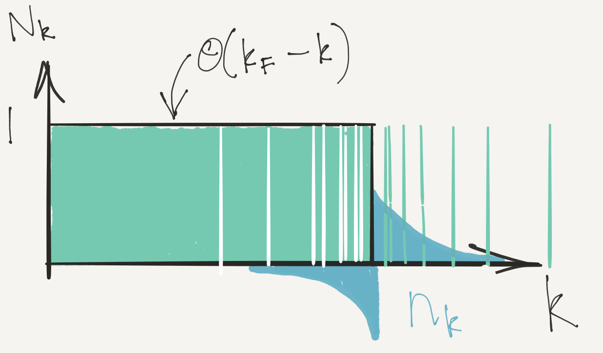
Ground state is Fermi sphere of radius $k_\text{F}$ in momentum space with $N_{s}(\bk) = \theta(k_F-\abs{\bk})$.
Low energy excited states will have $N_{s}(\bk)=1$ for $\abs{\bk}\ll k_\text{F}$ and $N_{s}(\bk)=0$ for $\abs{\bk}\gg k_\text{F}$.
In perturbation theory we can still label eigenstates by these occupation numbers even though eigenstates $\neq\ket{\mathbf{N}}$
- Without interaction energy of a state $\ket{\mathbf{N}}$ is
$$ E^{(0)}(\mathbf{N}) = \sum_{\bk,s} \epsilon(\bk)N_{s}(\bk) $$
For $U_0\neq 0$ energy $E(\mathbf{N})$ is function of labels, but no longer linear
Second order expansion of energy in terms of deviation of occupancies from ground state values is key ingredient of Landau’s theory
Perturbation Theory to Second Order
- Second order perturbation theory for the energies
$$ \begin{align*} E^{(1)}(\mathbf{N}) &= \braket{\mathbf{N}|H_\text{int}|\mathbf{N}}\\ E^{(2)}(\mathbf{N}) &= \sum_{\mathbf{N}'\neq \mathbf N}\frac{\abs{\braket{\mathbf{N'}|H_\text{int}|\mathbf{N}}}^2}{E^{(0)}(\mathbf{N})-E^{(0)}(\mathbf{N}')} \end{align*} $$
- First order correction is easy
$$ E^{(1)}(\mathbf{N}) = \frac{U_0}{V} \sum_{\bk,\bk'} N_{\uparrow}(\bk)N_{\downarrow}(\bk') = \frac{U_0}{V}N_\uparrow N_\downarrow. $$(energy used in Stoner criterion in Lecture 6)
- For second order we need
$\braket{\mathbf{N}'|H_\text{int}|\mathbf{N}}$, nonzero if$$ \begin{align*} N'_{\bk_1,\uparrow} = N_{\uparrow}(\bk_1) + 1, \quad N'_{\downarrow}(\bk_2) = N_{\downarrow}(\bk_2) + 1\\ N'_{\downarrow}(\bk_3) = N_{\downarrow}(\bk_3) - 1, \quad N'_{\uparrow}(\bk_4) = N_{\uparrow}(\bk_4) - 1, \end{align*} $$for $\bk_i$ satisfying $\bk_1+\bk_2=\bk_3+\bk_4$$$ \braket{\mathbf{N}'|H_\text{int}|\mathbf{N}} = \frac{U_0}{V} \left(1-N_{\uparrow}(\bk_1)\right)\left(1-N_{\downarrow}(\bk_2)\right)N_{\downarrow}(\bk_3)N_{\uparrow}(\bk_4) $$(ignoring any coinciding momenta; occupancies 0 or 1)
$$ E^{(2)}(\mathbf{N}) = \left(\frac{U_0}{V}\right)^2 \sum_{\bk_1+\bk_2=\bk_3+\bk_4}\frac{\left(1-N_{\uparrow}(\bk_1)\right)\left(1-N_{\downarrow}(\bk_2)\right)N_{\downarrow}(\bk_3)N_{\uparrow}(\bk_4)}{\epsilon(\bk_3)+\epsilon(\bk_4)-\epsilon(\bk_1)-\epsilon(\bk_2)} $$
Landau $f$ function
$E^{(2)}(\mathbf{N})$ has three independent momentum sums! 🙀
We are after excitation energies, so expand in change in occupation
$$ N_{s}(\bk) = \theta(k_F-\abs{\bk}) + n_{s}(\bk) $$
$n_\bk$is mean deviation from Fermi sphere in continuum limit:
- Excitation energy expanded in $n_\bk$
$$ \Delta E = \sum_{\bk,s} \varepsilon_s(\bk)n_{s}(\bk) + \frac{1}{2V}\sum_{\bk, s,\bk’, s’} f_{s^{}s’}(\bk,\bk’)n_{s}(\bk)n_{s’}(\bk’) $$
This is Landau’s key idea, not restricted to perturbation theory
At first order
$$ \begin{align*} \varepsilon_s(\bk) &= \epsilon(\bk) + \frac{U_0 N_{\bar s}}{V}+\cdots\\ f_{\uparrow\downarrow} &= f_{\downarrow\uparrow} = U_0+\cdots,\quad f_{\uparrow\uparrow}=f_{\downarrow\downarrow}=0+\cdots \end{align*} $$$\bar s$ is $\bar\uparrow=\downarrow$, $\bar\downarrow=\uparrow$ 🥱
- Second order contributions to $f$-function more interesting
$$ E^{(2)}(\mathbf{N}) = \left(\frac{U_0}{V}\right)^2 \sum_{\bk_1+\bk_2=\bk_3+\bk_4}\frac{\left(1-N_{\uparrow}(\bk_1)\right)\left(1-N_{\downarrow}(\bk_2)\right)N_{\downarrow}(\bk_3)N_{\uparrow}(\bk_4)}{\epsilon(\bk_3)+\epsilon(\bk_4)-\epsilon(\bk_1)-\epsilon(\bk_2)} $$
$$ N_{s}(\bk) = \theta(k_F-\abs{\bk}) + n_{s}(\bk) $$
$$ \begin{align*} f_{\uparrow\uparrow}(\bk,\bk') = -\frac{U_0^2}{V}\left[\sum_{\bk+\bk_3=\bk'+\bk_2} \frac{N_{\downarrow}(\bk_3)(1-N_{\downarrow}(\bk_2))}{\epsilon(\bk)+\epsilon(\bk_3)-\epsilon(\bk')-\epsilon(\bk_2)}\right.\nonumber\\ \left.+\sum_{\bk'+\bk_3=\bk+\bk_2}\frac{N_{\downarrow}(\bk_3)(1-N_{\downarrow}(\bk_2))}{\epsilon(\bk')+\epsilon(\bk_3)-\epsilon(\bk)-\epsilon(\bk_2)}\right] \end{align*} $$
- $f_{\uparrow\uparrow}(\bk,\bk’)$ is more complicated
$$ \begin{align*} f_{\uparrow\downarrow}(\bk,\bk') = U_0 + f_{\uparrow\uparrow}(\bk,\bk') +\frac{U_0^2}{V}\left[\sum_{\bk+\bk'=\bk_3+\bk_4}\frac{N(\bk_3)N(\bk_4)}{\epsilon(\bk_3)+\epsilon(\bk_4)-2E_\text{F}}\right.\nonumber\\ \left.\sum_{\bk+\bk'=\bk_1+\bk_2}\frac{(1-N(\bk_1))(1-N(\bk_2))}{2E_\text{F}-\epsilon(\bk_1)-\epsilon(\bk_2)}\right] \end{align*} $$(just for reference)
$n_{s}(\bk)\neq 0$ in energy window of size $k_\text{B} T$ around Fermi surface
At low $T$ take
$\abs{\bk}=\abs{\bk'}=k_\text{F}$. New feature at second order is nontrivial dependence of $f_{s^{}s’}(\bk,\bk’)$ on angle between $\bk$ and $\bk’$.Assume ground state unpolarized, i.e. $N_{s}(\bk)$ independent of $s$
It’s a bit fiddly to get at, but let’s work it out for the simpler case of $f_{\uparrow\uparrow}(\bk,\bk’)$! (only have one independent momentum 😀)
Continuum limit
$$ \begin{align*} f_{\uparrow\uparrow}(\bk,\bk') = \frac{U_0^2}{(2\pi)^3}\left[\int_{\substack{\abs{\bk_3}<k_\text{F},\abs{\bk_2}>k_\text{F}\\ \bk+\bk_3=\bk'+\bk_2 }} \frac{d\bk_3}{\epsilon(\bk_2)-\epsilon(\bk_3)} +\int_{\substack{\abs{\bk_3}<k_\text{F},\abs{\bk_2}>k_\text{F}\\ \bk'+\bk_3=\bk+\bk_2 }}\frac{d\bk_3}{\epsilon(\bk_2)-\epsilon(\bk_3)}\right] \end{align*} $$
- Need integral
$$ \int_{\substack{\abs{\bk_3}<k_\text{F},\abs{\bk_2}>k_\text{F}\\ \bk+\bk_3=\bk'+\bk_2 }} \frac{d\bk_3}{\epsilon(\bk_2)-\epsilon(\bk_3)} $$
Denominator can be written ($\bk-\bk’$ is fixed) $$ \epsilon(\bk_2)-\epsilon(\bk_3)= \frac{1}{2m}\left(\bk_2+\bk_3\right)\cdot\left(\bk_2-\bk_3\right) = \frac{1}{2m}\left(\bk_2+\bk_3\right)\cdot\left(\bk-\bk’\right) $$
Notation $\mathbf{K} = \frac{1}{2}\left(\bk_2+\bk_3\right),\quad \bq = \frac{1}{2}\left(\bk_2-\bk_3\right)$
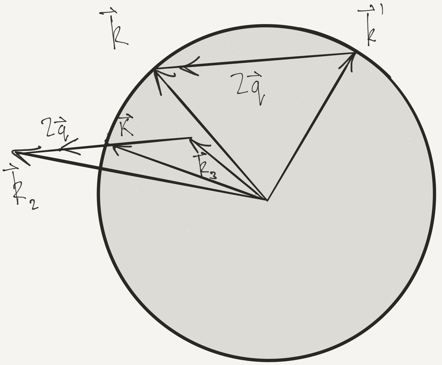
Denominator becomes (for fixed $\bq$) $$ \epsilon(\bk_2)-\epsilon(\bk_3) = \frac{2}{m}\mathbf{K}\cdot\bq $$
Only angle $\theta$ between $\mathbf{K}$ and $\bq$ enters integral
Conditions $\abs{\bk_2}>k_\text{F}$ and $\abs{\bk_3}<k_\text{F}$ become $$ \begin{align*} \left(\mathbf{K}+\bq\right)^2>k_\text{F}^2,\quad \left(\mathbf{K}-\bq\right)^2<k_\text{F}^2 \end{align*} $$ which gives range of $K_-(\theta)<\abs{\mathbf{K}}<K_+(\theta)$ $$ K_{\pm}(\theta)=\pm q\abs{\cos\theta}+\sqrt{k_\text{F}^2-q^2\sin^2\theta},\qquad \theta<\pi/2 $$
- In terms of these variables
$$ \begin{align*} \int_{\substack{\abs{\bk_3}<k_\text{F},\abs{\bk_2}>k_\text{F}\\ \bk+\bk_3=\bk'+\bk_2 }} \frac{d\bk_3}{\epsilon(\bk_2)-\epsilon(\bk_3)}&= \pi m\int_0^{\pi/2} d\theta \int_{K_-(\theta)}^{K_+(\theta)} \frac{K\sin\theta}{q\cos\theta} dK\nonumber\\ &=2\pi m\int_0^{\pi/2} d\theta \sin\theta \sqrt{k_\text{F}^2-q^2\sin^2\theta} \end{align*} $$
- Other integral is same but in interval $(\pi/2,\pi)$. Finally…
$$ \begin{align*} f_{\uparrow\uparrow}(\bk,\bk') &= \frac{U_0^2 m}{(2\pi)^2} \int_0^{\pi} d\theta \sin\theta \sqrt{k_\text{F}^2-q^2\sin^2\theta}\nonumber\\ &=\frac{U_0^2 m k_\text{F}}{(2\pi)^2}\left[1 - \frac{\cos^2\phi/2}{2\sin\phi/2}\log\left(\frac{1-\sin\phi/2}{1+\sin\phi/2}\right)\right] \end{align*} $$$\phi$ is the angle between $\bk$ and$\bk'$i.e.$\abs{\bk-\bk'}=2q=2k_\text{F}\sin\phi/2$
Our definition of $f$ implied quantization axis for spin
To write things in invariant way, think of occupation number $N(\bk)$ as $2\times 2$ matrix
$$ \mathsf{N}(\bk)=\begin{pmatrix} N_{\uparrow\uparrow}(\bk) & N_{\uparrow\downarrow}(\bk) \\ N_{\downarrow\uparrow}(\bk) & N_{\downarrow\downarrow}(\bk). \end{pmatrix} $$
- $f$-function then has four spin indices
$$ \frac{1}{2V}\sum_{\bk, s_1,s_2,\bk', s_3,s_4} f_{s_1s_2,s_3s_4}(\bk,\bk')n_{s_1s_2}(\bk)n_{s_3s_4}(\bk'), $$
$$ \begin{align*} f_{s_1s_2,s_3s_4}(\bk,\bk') = \frac{U_0}{2}\left[\left(1+ \frac{mU_0 k_\text{F}}{2\pi^2}\left[2+\frac{\cos\phi}{2\sin\phi/2}\log\frac{1+\sin\phi/2}{1-\sin\phi/2}\right]\right)\delta_{s_1s_3}\delta_{s_2s_4}\right.\nonumber\\ \left.\left(1+ \frac{mU_0 k_\text{F}}{2\pi^2}\left[1-\frac{1}{2}\sin\phi/2\log\frac{1+\sin\phi/2}{1-\sin\phi/2}\right]\right)\boldsymbol{\sigma}_{s_1s_3}\cdot\boldsymbol{\sigma}_{s_2s_4}\right] \end{align*} $$
(again, just for reference)
- Key message: interaction between quasiparticles in an interacting Fermi gas is defined in terms of a pair of functions
$$ \nu(E_F)f_{s_1s_2,s_3s_4}(\bk,\bk') = F(\phi) \delta_{s_1s_3}\delta_{s_2s_4} + G(\phi)\boldsymbol{\sigma}_{s_1s_3}\cdot\boldsymbol{\sigma}_{s_2s_4} $$ - $F(\phi)$ and $G(\phi)$ made dimensionless by scaling by density of states at Fermi surface $\nu(E_F)\equiv k_{\text{F}}m/\pi^2$.
Quasiparticle energy $\varepsilon_s(\bk)$
$$ \Delta E = \sum_{\bk,s} \varepsilon_s(\bk)n_{s}(\bk) + \frac{1}{2V}\sum_{\bk, s,\bk’, s’} f_{s^{}s’}(\bk,\bk’)n_{s}(\bk)n_{s’}(\bk’). $$
$\varepsilon_s(\bk)$ will involve two momentum sums 😟
What can we say on general grounds? Near Fermi surface expect
$$ \varepsilon_s(\bk) - E_\text{F} \approx v_\text{F}(\abs{\bk}-k_\text{F}) $$
- Fermi velocity
$v_\text{F}$altered by interactions. Define effective mass
$$ m_* = \frac{k_\text{F}}{v_\text{F}} $$
Can get $m_*$ using results we have alrady, using one simple trick
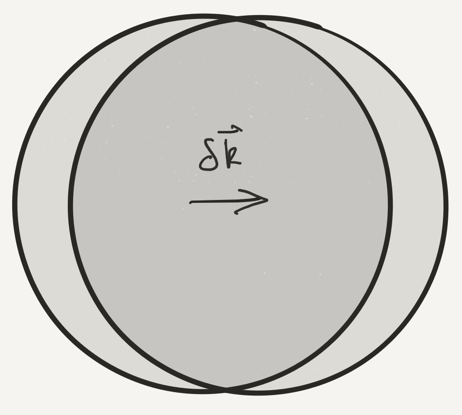
Shift momentum of each quasiparticle by $\delta\bk$, giving new $N_s(\bk)$
$$ \begin{align*} N_s(\bk-\delta\bk) &=\theta(k_F-\abs{\bk-\delta\bk}) + n_{s}(\bk-\delta\bk)+\cdots\nonumber\\ &=\theta(k_F-\abs{\bk}) + n_s(\bk) + \delta(k_F-\abs{\bk})\hat\bk\cdot\delta\bk - \delta\bk \nabla_\bk n_{s}(\bk)+\cdots. \end{align*} $$
- Compute energy using Landau functional
$$ \begin{align*} N_s(\bk-\delta\bk) &=\theta(k_F-\abs{\bk}) + n_s(\bk) + \delta(k_F-\abs{\bk})\hat\bk\cdot\delta\bk - \delta\bk \nabla_\bk n_{s}(\bk)+\cdots. \end{align*} $$
- Treat last three terms as $n_s(\bk)$. Excitation energy changes
$$ \begin{align*} \Delta E(\text{after})-\Delta E(\text{before}) = \sum_{\bk,s} n_{s}(\bk)\delta\bk\cdot\nabla_\bk\varepsilon_s(\bk) \nonumber\\ +\frac{1}{V}\sum_{\bk, s,\bk', s'} f_{s^{}s'}(\bk,\bk')n_{s}(\bk)\left[\delta(k_F-\abs{\bk'})\hat\bk'\cdot\delta\bk - \nabla_{\bk'}n_{s'}(\bk')\cdot\delta\bk\right]. \end{align*} $$(to first order in $\delta\bk$. Integrate by parts in first term)
- On grounds of Galilean invariance, this change must be $$ \Delta E(\text{after})-\Delta E(\text{before}) = \frac{\mathbf{P}}{m}\cdot\delta\bk $$ where total momentum $\mathbf{P}$ is
$$ \mathbf{P} = \sum_{\bk,s} \bk n_{s}(\bk). $$
- If two expressions for $\Delta E(\text{after})-\Delta E(\text{before})$ equal for all $n_s(\bk)$ and $\delta\bk$ to first order
$$ \frac{\bk}{m} = \nabla_\bk\varepsilon_s(\bk) + \sum_{s'}\int f_{s^{}s'}(\bk,\bk')\delta(k_F-\abs{\bk'})\hat\bk' \frac{d\bk'}{(2\pi)^3} $$
- For momenta close to the Fermi surface
$$ \frac{\bk}{m} = \frac{\bk}{m_*} +\frac{1}{m} \int F(\phi) \bk' \frac{d\Omega_{\bk'}}{4\pi} $$
- If
$\bk'=\cos\phi \bk + \sin\phi \bk_\perp$, with $\bk_\perp\cdot\bk=0$, we get
$$ \frac{1}{m} = \frac{1}{m_*} +\frac{1}{m} \int F(\phi) \cos\phi \frac{\sin\phi d\phi}{2} $$
For the $F(\phi)$ that we found in $2^{\text{nd}}$ order perturbation theory $$ \frac{m_*}{m} = 1 + \frac{1}{30\pi^4}(7\log 2 - 1)\left(mU_0k_\text{F}\right)^2+\cdots. $$ (Use the substitution $u=\sin\phi/2$ to do the integral.)
In systems with strong interactions $m_*/m$ may be much larger!
In heavy fermion materials $m_*/m$ can approach 1000! Landau’s picture of fermionic quasiparticles still applies.
Eigenstates in Perturbation Theory: What is a Quasiparticle?
What do these quasiparticle states look like? Let’s see what perturbation theory says
At first order we have
$$ \ket{\mathbf{N}^{(1)}} = \sum_{\mathbf{N}'\neq \mathbf N}\frac{\braket{\mathbf{N'}|H_\text{int}|\mathbf{N}}}{E^{(0)}(\mathbf{N})-E^{(0)}(\mathbf{N}')}\ket{\mathbf{N}'} $$
Consider the Fermi sea ground state $\ket{\text{FS}}$. What states
$\ket{\mathbf{N'}}$can appear this case?Only possibility is that the interaction creates two particle-hole pairs out of the Fermi sea, with total momentum zero.
What about an excited state? If we consider the state $$ \adop_{\bk,s}\ket{\text{FS}} $$ two kinds of states can contribute
Create a pair of particle-hole pairs
Create a single particle-hole pair and move particle at $\bk$

Consider
$\adop_{\bk,s}\ket{0}$, creating a particle in exact ground stateSince $\ket{0}$ includes the first type of state (2 particle-hole pair states), $\adop_{\bk,s}\ket{0}$ is only missing second kind
Single quasiparticle state is
$$ \begin{align*} \ket{\bk,s} &= \sqrt{\frac{z_k}{\braket{0|\aop_{\bk,s}\adop_{\bk,s}|0}}}\adop_{\bk,s}\ket{0} \\ &+ \frac{U_0}{V}\sum_{\substack{\bk_1+\bk_2=\bk_3+\bk\\ s,s'}}\frac{\adop_{\bk_1,s}\adop_{\bk_2,s'}\aop_{\bk_3,s'}\ket{\text{FS}}}{\epsilon(\bk_1)+\epsilon(\bk_2)-\epsilon(\bk_3)-\epsilon(\bk)} \end{align*} $$$\sqrt{z_k}$ is a normalization factor
Normalizing, $1-z_\bk$ is
$$ \begin{align*} \left(\frac{U_0}{V}\right)^2\sum_{\substack{\bk_1+\bk_2=\bk_3+\bk\\\abs{\bk_3}<k_\text{F},\abs{\bk_2},\abs{\bk_1}>k_\text{F}\\ s,s'}}\frac{1}{\left[\epsilon(\bk_1)+\epsilon(\bk_2)-\epsilon(\bk_3)-\epsilon(\bk)\right]^2}+\cdots \end{align*} $$
- This is overlap of single quasiparticle state $\ket{\bk,s}$ with $\adop_{s,\bk}\ket{0}$.
$$ z_\bk = \frac{\abs{\braket{\bk,s|\adop_{\bk,s}|0}}^2}{\braket{0|\aop_{\bk,s}\adop_{\bk,s}|0}} $$
A finite overlap – for quasiparticles at the Fermi surface – is requirement for Fermi liquid picture to hold
If it were to vanish, any resemblance of the quasiparticle to a free fermion would disappear!
For our example (hard!): $$ z_{\abs{\bk}=k_\text{F}} = 1 - \frac{(mUk_\text{F})^2}{8\pi^4}\left[\log 2 + \frac{1}{3}\right] $$
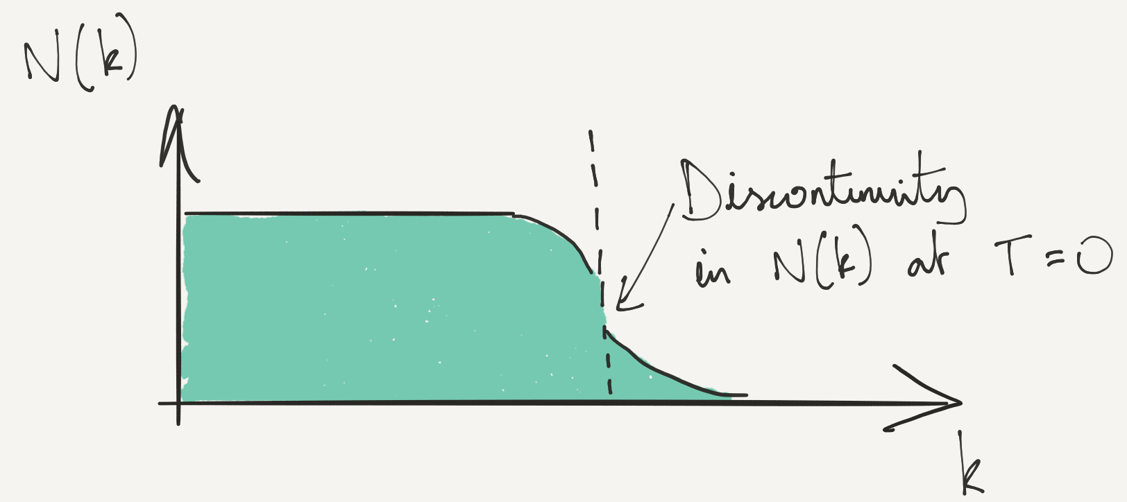
This is also the occupation number of the original fermions $\braket{0|\adop_{\bk,s}\aop_{\bk,s}|0}$ (not the quasiparticles!) just below the Fermi surface in the ground state (see Problem Set 3. There is a corresponding result just above. Even with interactions, there is a finite step in the distribution function at the Fermi surface.