Spin Models

Up to now our degrees of freedom have been particles
In this lecture: systems of interacting spins

$$ \nonumber \newcommand{\cN}{\mathcal{N}} \newcommand{\br}{\mathbf{r}} \newcommand{\bp}{\mathbf{p}} \newcommand{\bk}{\mathbf{k}} \newcommand{\bq}{\mathbf{q}} \newcommand{\bv}{\mathbf{v}} \newcommand{\pop}{\psi^{\vphantom{\dagger}}} \newcommand{\pdop}{\psi^\dagger} \newcommand{\Pop}{\Psi^{\vphantom{\dagger}}} \newcommand{\Pdop}{\Psi^\dagger} \newcommand{\Phop}{\Phi^{\vphantom{\dagger}}} \newcommand{\Phdop}{\Phi^\dagger} \newcommand{\phop}{\phi^{\vphantom{\dagger}}} \newcommand{\phdop}{\phi^\dagger} \newcommand{\aop}{a^{\vphantom{\dagger}}} \newcommand{\adop}{a^\dagger} \newcommand{\bop}{b^{\vphantom{\dagger}}} \newcommand{\bdop}{b^\dagger} \newcommand{\cop}{c^{\vphantom{\dagger}}} \newcommand{\cdop}{c^\dagger} \newcommand{\bra}[1]{\langle{#1}\rvert} \newcommand{\ket}[1]{\lvert{#1}\rangle} \newcommand{\inner}[2]{\langle{#1}\rvert #2 \rangle} \newcommand{\braket}[3]{\langle{#1}\rvert #2 \lvert #3 \rangle} \newcommand{\sgn}{\mathrm{sgn}} \newcommand{\brN}{\br_1, \ldots, \br_N} \newcommand{\xN}{x_1, \ldots, x_N} \newcommand{\zN}{z_1, \ldots, z_N} $$

Ising Model

$$ H = J\sum_{\langle j,k\rangle} \sigma_j \sigma_k, \label{spin_ising} $$

‘spin’ variables $\sigma_j=\pm 1$
${\langle j,k\rangle}$ indicates sum over nearest neighbour pairs
$J<0$ favours aligned spins, leading to ferromagnetism

But… not really a quantum model

$N$ spin-1/2: states and operators

1 spin-1/2: $\psi_{\pm}$ in $s^z$ basis (say). $N$-spins: $\Psi_{\sigma_1,\ldots \sigma_N}$ has $2^N$ components
Product states $\ket{\sigma_1}\ket{\sigma_2}\cdots \ket{\sigma_N}$ form a basis

$$ \ket{\Psi}=\sum_{{\sigma_j=\pm}}\Psi_{\sigma_1\cdots \sigma_N}\ket{\sigma_1}\ket{\sigma_2}\cdots \ket{\sigma_N} $$

Tensor product

For (distinguishable) particles product states were

$$ \label{quantum_statistics_disting} \Psi_{\alpha_{1}\alpha_{2}\cdots \alpha_{N}}(\br_1,\ldots \br_N)=\varphi_{\alpha_{1}}(\mathbf{r_{1}})\varphi_{\alpha_{2}}(\mathbf{r_{2}})\cdots\varphi_{\alpha_{N}}(\mathbf{r_{N}}) $$

Abstract form

$$ \ket{\Psi_{\alpha_{1}\alpha_{2}\cdots \alpha_{N}}}=\ket{\varphi_{\alpha_{1}}}\ket{\varphi_{\alpha_{2}}}\cdots\ket{\varphi_{\alpha_{N}}} $$

This is a tensor product, normally denoted

$$ \ket{\Psi_{\alpha_{1}\alpha_{2}\cdots \alpha_{N}}}=\ket{\varphi_{\alpha_{1}}}\otimes\ket{\varphi_{\alpha_{2}}}\cdots\otimes\ket{\varphi_{\alpha_{N}}} $$

We drop the $\otimes$ for brevity

Operators

Spin operators obey $[s^a,s^b]=i\epsilon_{abc}s^c$
A spin operator $s^a_j$ acts on $j^\text{th}$ spin

$$ s^a_j\ket{\sigma_1}\ket{\sigma_2}\cdots \ket{\sigma_N} = \ket{\sigma_1}\ket{\sigma_2}\cdots \ket{\sigma_{j-1}} (s^a \ket{\sigma_j}) \ket{\sigma_{j+1}}\cdots\ket{\sigma_N} $$

Which is the same as

$$ s^a_j = \overbrace{\mathbb{1}\otimes \cdots \mathbb{1}}^{j-1}\otimes s^a \otimes \overbrace{\mathbb{1} \otimes\cdots \mathbb{1}}^{N-j} $$

What is $[s^a_j,s^b_k]$ for $j\neq k$?

Ising model Hamiltonian

$$ H = 4J\sum_{\langle j,k\rangle} s^z_j s^z_k $$

Eigenstates are product states $\ket{\sigma_1}\ket{\sigma_2}\cdots \ket{\sigma_N}$ with energy

$$ E_{\sigma_1\cdots \sigma_N} = J\sum_{\langle j,k\rangle} \sigma_j \sigma_k $$

Fine for statistical mechanics but a bit boring for QM!

Heisenberg Model

More realistic

$$ H = J \sum_{\langle j,k\rangle} \mathbf{s}_j \cdot \mathbf{s}_k. \label{spin_Hberg} $$

$\left[s^a_j,s^b_k\right]=i\delta_{jk}\epsilon_{abc}s^c_j$
Unlike the elastic lattice, not possible to solve in general
Captures many of the dynamical features (e.g. spin waves) of real magnetic materials.

Heisenberg Ferromagnetic Chain

Begin with the 1D case

$$ H = J \sum_{j=1}^N \mathbf{s}_j \cdot \mathbf{s}_{j+1}, $$

As usual $\mathbf{s}_j=\mathbf{s}_{j+N}$ (periodic boundary conditions).
Some anisotropic materials have magnetic atoms arranged in weakly coupled chains

It’s often useful to write $$ \mathbf{s}_j \cdot \mathbf{s}_{j+1} = s^z_js^z_{j+1} + \frac{1}{2}\left(s^+_js^-_{j+1} +s^-_js^+_{j+1}\right), $$ where $s^\pm = s^x\pm i s^y$ $$ s^+ = \begin{pmatrix} 0 & 1 \\ 0 & 0 \end{pmatrix},\qquad s^- = \begin{pmatrix} 0 & 0 \\ 1 & 0 \end{pmatrix} $$ are the spin raising and lowering operators

Ground state for $J<0$

$$ \ket{\text{FM}} \equiv \ket{+}_1 \ket{+}_2 \cdots \ket{+}_N $$

Show that this is eigenstate of $H$ with $E_0\equiv JN/4$

Also eigenstate of $S^z$ and $\mathbf{S}^2$, where $\mathbf{S}$ is total spin

$$ \mathbf{S} = \sum_{j=1}^N \mathbf{s}_j=(S^x, S^y, S^z) $$

Eigenvalues are $S^z = N/2$ and $\mathbf{S}^2 = \frac{N}{2}\left(\frac{N}{2}+1\right)$.

Ground state multiplet

Rotational invariance implies that $\ket{\text{FM}}$ is member of multiplet of $N+1$ degenerate eigenstates related by rotations
These states can be generated by acting with $S^-=S^x-iS^y$ $$ S^-\ket{\text{FM}} = \sum_{j=1}^N s^-_j\ket{\text{FM}} = \sum_{j=1}^N \ket{+}_1\ket{+}_2\cdots \ket{+}_{j-1} \ket{-}_j\ket{+}_{j+1}\cdots \ket{+}_N. \label{spin_Lowered} $$

$S^z = N/2-1$, but $\mathbf{S}^2$ and $H$ unchanged.

$\left(S^-\right)^2\ket{\text{FM}}$ is constant amplitude superposition of states with two spins flipped, etc.

First Excited States

What about?

$$ \ket{j} = \ket{+}_1\ket{+}_2\cdots \ket{+}_{j-1} \ket{-}_j\ket{+}_{j+1}\cdots \ket{+}_N. $$

Is this an eigenstate? Act with Hamiltonian, using

$$ \mathbf{s}_j \cdot \mathbf{s}_{j+1} = s^z_js^z_{j+1} + \frac{1}{2}\left(s^+_js^-_{j+1} +s^-_js^+_{j+1}\right), $$

Now note that

$$ \left(s^+_j s^-_{j+1} +s^-_js^+_{j+1}\right)\ket{+}_j\ket{-}_{j+1} = \ket{-}_j\ket{+}_{j+1}. $$

Action of $H$ on $\ket{j}$ is $$ H\ket{j} = (1-N/4) \ket{j} - \frac{1}{2}\left(\ket{j-1}+\ket{j+1}\right). $$ (set $J=-1$ from now)
Leaves us in subspace spanned by states $\ket{j}$: this is subspace with $S_z=N/2-1$
Flips are like particles (magnons), with Hamiltonian conserving number

Eigenstates are plane waves $$ H\ket{j} = (1-N/4) \ket{j} - \frac{1}{2}\left(\ket{j-1}+\ket{j+1}\right). $$ $$ \begin{equation} \ket{\eta} = \frac{1}{\sqrt{N}}\sum_{j=1}^N e^{i\eta j}\ket{j}, \qquad \eta = \frac{2\pi n}{N} \end{equation} $$
Eigenvalues $E = E_0 + \omega(\eta)$

$$ \omega(\eta) = 2\sin^2\eta/2. \label{spin_dispersion} $$

Dispersion is periodic, as for elastic chain, but quadratic, rather than linear, at small $\eta$
$\eta=0$ corresponds to the state $S^-\ket{\text{FM}}$

$N$-Magnon States

A magnon has energy $\propto J$
System with extensive energy / finite temperature must have many magnons
Dimension of subspace of $n$ flipped spins is $\binom{N}{n}$
Magnons can’t sit on the same site. Things get difficult!

Antiferromagnets Are Different!

Let’s try and guess the ground state for $J>0$
Since anti-aligning spins should be favoured, we might try $$ \ket{\text{AFM}} \equiv \ket{+}_1\ket{-}_{2}\cdots \ket{+}_{N-1}\ket{-}_{N}, \label{spin_AFM} $$
What does $H$ do? Remember $$ \mathbf{s}_j \cdot \mathbf{s}_{j+1} = s^z_js^z_{j+1} + \frac{1}{2}\overbrace{\left(s^+_js^-_{j+1} +s^-_js^+_{j+1}\right)}^{\text{swaps }\ket{+}_j\ket{-}_{j+1}}, $$ spin flip terms cause spins to move about. Ground state is more complicated!

For the AFM chain, quantum fluctuations too strong for AFM order
Antiferromagnets do exist in higher dimensions, and Néel state $\ket{\text{AFM}}$ is good starting approximation

Large $s$ Expansion

Generalize model to $s>1/2$ (magnetic ions can have higher spin)
Develop approximations that work for $s\gg 1/2$
Hope that the qualitative behaviour we find holds for $s=1/2$

Holstein–Primakoff Representation

Represent spins as oscillators!
Coupled spins becomes coupled oscillators
Representation not linear, so we get anharmonic chain
Harmonic approximation justified when spin large

$$ \begin{align} s^+ &=\sqrt{2s}\sqrt{1-\frac{\adop\aop}{2s}}\aop \\ s^- &= \sqrt{2s}\adop\sqrt{1-\frac{\adop\aop}{2s}} \\ s^z &= \left(s - \adop \aop\right). \end{align} $$

Show that $[\aop,\adop]=1$ reproduces the spin commutation relations $[s^a,s^b]=i\epsilon_{abc}s^c$

One way to think of it…

$s^{\pm}$ and $\aop$, $\adop$ both shift us up and down a ladder of states. $$ s^\pm\ket{s,m} = \sqrt{s(s+1)-m(m\pm 1)}\ket{s,m\pm 1} $$ Relation between $s^z$ and number of quanta $n$ is simple: $s^z = s - n$
Difference: $2s+1$ spin states, but infinite oscillator states
$s^+\propto \aop$, $s^-\propto \adop$ doesn’t work. Something needed to stop us lowering beyond $s^z=-s$ $$ s^- = \sqrt{2s}\adop\sqrt{1-\frac{\adop\aop}{2s}} $$

Another way…

drawing

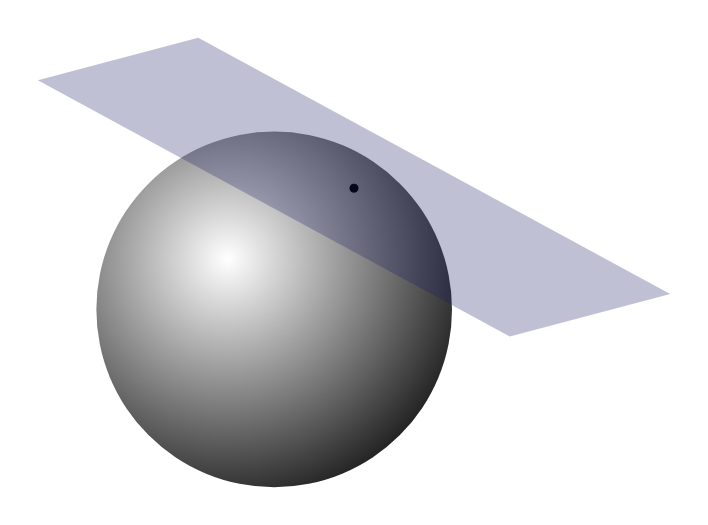
Classical spin described by point on sphere of radius $\sim s$
Large $s$: approximate locally by plane
Near north pole $[s^x,s^y]=is^z\sim is$ resembles $[x,p]=i$
Therefore $s^\pm$ resemble $\aop$, $\adop$

Harmonic Spin Waves

Large $s$ approximation $$ \begin{align} s^+ &\sim \sqrt{2s}\aop \qquad s^- \sim \sqrt{2s}\adop \qquad s_z = \left(s - \adop \aop\right). \label{spin_HPapprox} \end{align} $$ neglecting terms of order $s^{-1/2}$.
Heisenberg Hamiltonian becomes quadratic oscillator Hamiltonian $$ \begin{align} s^x &\sim \sqrt{s}x \nonumber\\ s^y &\sim \sqrt{s}p\nonumber\\ s_z &= \left(s - \frac{1}{2}[x^2 + p^2 - 1] \right), \end{align} $$ where $x = \frac{1}{\sqrt{2}}(\aop+\adop)$ and $p = \frac{i}{\sqrt{2}}(\adop-\aop)$

$$ \begin{align} s^x &\sim \sqrt{s}x \nonumber\\ s^y &\sim \sqrt{s}p\nonumber\\ s_z &= \left(s - \frac{1}{2}[x^2 + p^2 - 1] \right), \end{align} $$

$$ H = J \sum_{j=1}^N \mathbf{s}_j \cdot \mathbf{s}_{j+1} $$

$$ H\sim NJ s^2 + sNJ+ \overbrace{sJ \sum_{j=1}^N \left[x_j x_{j+1} + p_j p_{j+1}-x_j^2 - p_j^2\right]}^{\equiv H^{(2)}} + \ldots, \label{spin_Harmonic} $$

Use Fourier expansion of the position and momentum $$ \begin{align} x_j(t) &= \frac{1}{\sqrt{N}}\sum_{|n| \leq (N-1)/2} q_n(t) e^{i\eta_n j},\nonumber\\ p_j(t) &= \frac{1}{\sqrt{N}}\sum_{|n| \leq (N-1)/2} \pi_n(t) e^{-i\eta_n j}\\ H^{(2)} &= -2sJ \sum_{|n| \leq (N-1)/2} \sin^2(\eta_n/2)\left[q_n q_{-n} + \pi_n\pi_{-n}\right] \end{align} $$
We can read off dispersion $$ \omega_{\text{FM}}(\eta) = 4s\left|J\right|\sin^2(\eta/2) $$ c.f. $\omega(\eta) = 2\sin^2\eta/2$ that we found for $s=1/2$

$$ H\sim NJ s^2 + sNJ+ \overbrace{ -2sJ \sum_{|n| \leq (N-1)/2} \sin^2(\eta_n/2)\left[q_n q_{-n} + \pi_n\pi_{-n}\right]}^{\equiv H^{(2)}} + \ldots, $$

Ground state energy of $H^{(2)}$ is

$$ -2sJ\sum_{|n| \leq (N-1)/2} \frac{1}{2}\sin^2(\eta_n/2) = -sJN $$

Overall $E_0 = NJs^2$, which is exact energy of $\ket{FM}$

AFM case

Close to $\ket{\text{FM}}$ few oscillator quanta; harmonic approximation OK
Classically, small amplitude nonlinear oscillations treated as linear
What about AFM case? Make it look like FM
Rotate every other spin through $\pi$ about the $y$ axis, so that

$$ (s^x_j,s^y_j,s^z_j)\longrightarrow (-s^x_j,s^y_j,-s^z_j),\quad j\text{ odd}. $$

The Heisenberg chain Hamiltonian becomes $$ H = -J \sum_{j=1}^N \left[s^x_j s^x_{j+1} - s^y_j s^y_{j+1} + s^z_j s^z_{j+1}\right]. $$

Harmonic approximation means: close to AFM in original variables
Oscillator Hamiltonian is now $$ H^{(2)} = 2sJ \sum_{|n| \leq (N-1)/2} \left[\sin^2(\eta/2)q_n q_{-n} + \cos^2(\eta/2)\pi_n\pi_{-n}\right], \label{spin_H2AFM} $$ corresponding to a dispersion relation

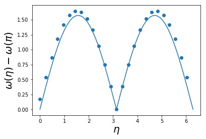
$$ \omega_{\text{AFM}}(\eta) = 2sJ\left|\sin(\eta)\right|. \label{spin_AFMDispersion} $$

$$ \omega_{\text{AFM}}(\eta) = 2sJ\left|\sin(\eta)\right|. $$

Vanishes at both $\eta=0$ and Brillouin zone boundary $\eta=\pi$
Linear near both points, c.f. quadratic for FM
Compare $$ H_\text{FM}^{(2)} = -2sJ \sum_{|n| \leq (N-1)/2} \sin^2(\eta_n/2)\left[q_n q_{-n} + \pi_n\pi_{-n}\right] $$ In FM both position and momentum terms vanish at $\eta=0$. This is the origin of quadratic dispersion at small $\eta$
In AFM position term vanishes at $\eta=0$, with momentum term vanishing at $\eta=\pi$. This gives linear dispersion at these points

$$ \omega_{\text{AFM}}(\eta) = 2sJ\left|\sin(\eta)\right|. $$

We know (by other means) exact dispersion relation for lowest excited state of momentum $\eta$ (des Cloiseaux–Pearson mode) $$ \omega_{\text{dCP}}(\eta) = \frac{\pi J}{2}\left|\sin(\eta)\right|, \label{spin_dCP} $$ Same functional form, but with a different overall scale

drawing

Ground state fluctuations

Crudest approximation

$$ \bra{\text{FM}}s_j^z \ket{\text{FM}} = s, \qquad \bra{\text{AFM}}s_j^z \ket{\text{AFM}} = s(-1)^j $$

However, in Holstein–Primakoff representation

$$ s^z_j = s - \adop_j\aop_j. $$

How does second term effect $\bra{0}s^z_j \ket{0}$ in ground state of $H^{(2)}$?
We know it doesn’t for FM, because $\ket{\text{FM}}=\ket{0}$

$$ s^z_j = s - \adop_j\aop_j. $$

Why doesn’t second term contribute? By translational invariance

$$ \begin{align} \bra{0}\adop_j \aop_j\ket{0} &= \bra{0}\frac{1}{N}\sum_{j=1}^N \adop_j \aop_j\ket{0}\\ \sum_{j=1}^N \adop_j \aop_j &= \frac{1}{2} \sum_{j=1}^N \left(x_j^2 + p_j^2 - 1\right) = -\frac{N}{2} + \frac{1}{2}\sum_n \left(q_n q_{-n} + \pi_n\pi_{-n}\right). \end{align} $$

commutes with $$ H_\text{FM}^{(2)} = -2sJ \sum_{|n| \leq (N-1)/2} \sin^2(\eta_n/2)\left[q_n q_{-n} + \pi_n\pi_{-n}\right] $$ and is zero in the ground state (c.f. ground state energy)

AFM case

$$ s^z_j = (-1)^j(s-\adop_j\aop_j) $$

$q_n q_{-n} + \pi_n\pi_{-n}$ doesn’t commute with $\sin^2(\eta/2)q_n q_{-n} + \cos^2(\eta/2)\pi_n\pi_{-n}$
Express both in oscillator variables

$$ \begin{align} &\aop_\eta = \sqrt{\frac{|\tan(\eta /2)|}{2}}\left(q_n + \frac{i}{|\tan(\eta /2)|}\pi_{-n}\right)\nonumber\\ &\adop_\eta = \sqrt{\frac{|\tan(\eta /2)|}{2}}\left(q_{-n} - \frac{i}{|\tan(\eta /2)|}\pi_{n}\right),\qquad \eta=2\pi n/N \\ &\sin^2(\eta/2)q_n q_{-n} + \cos^2(\eta/2)\pi_n\pi_{-n}=\frac{\omega(\eta)}{2}\left[\adop_\eta\aop_\eta+\aop_\eta\adop_\eta\right]. \end{align} $$

To evaluate $\Delta s = \bra{0}\adop_j\aop_j\ket{0}$ write in terms of $\adop_\eta$, $a_\eta$

$$ \begin{align} \frac{1}{N}\sum_{j=1}^N \adop_j \aop_j &= \frac{1}{2N} \sum_{j=1}^N \left(x_j^2 + p_j^2 - 1\right) \\ &= -\frac{1}{2} + \frac{1}{2N}\sum_n \left(q_n q_{-n} + \pi_n\pi_{-n}\right) \end{align} $$ $$ \begin{align} \Delta s &= -\frac{1}{2}+\frac{1}{4N}\sum_n \left[|\tan(\eta_n/2)| + |\cot(\eta_n/2)|\right].\\ &= -\frac{1}{2}+\frac{1}{4}\int_{-\pi}^\pi \frac{d\eta}{2\pi} \left[|\tan(\eta_n/2)| + |\cot(\eta_n/2)|\right]. \end{align} $$

Integral diverges logarithmically at $\eta=0$ and $\eta=\pi$.

What went wrong? Our replacement $$ \sum_n (\ldots) \longrightarrow \frac{N}{2\pi}\int_{-\pi}^\pi (\ldots)d\eta $$ failed us because the summand is singular (c.f. $\langle (u_i-u_j)^2\rangle$ in the elastic chain)
At finite $N$ the sums are all finite if $\eta=0, \pi$ are excluded

$$ \Delta s \propto \log N $$

No AFM in 1D at zero temperature in $N\to\infty$ limit

Repeat the analysis on a 2D square lattice. You should find an integral over the two-dimensional Brillouin zone. Do you find divergences?