Chaos and information in
space-time dual classical circuits
Austen Lamacraft (Cambridge) and Pieter Claeys (Dresden)
austen.uk/#talks for slides
Dual unitaries and their phenomenology

Expectation values
- Evaluate $\bra{\Psi}\mathcal{O}\ket{\Psi}=\bra{\Psi_0}\mathcal{U}^\dagger\mathcal{O}\mathcal{U}\ket{\Psi_0}$ for local $\mathcal{O}$
Folded picture
- After folding, lines correspond to two indices / 4 dimensions
Unitarity in folded picture
- Circle denotes $\delta_{ab}$
$\bra{\Psi}\mathcal{O}\ket{\Psi}$ in folded picture
- Emergence of “light cone”
Reduced density matrix
- Expectation values in region $A$ evaluated using reduced density matrix
$$ \rho_A = \operatorname{tr}_{\bar A}\left[\ket{\Psi}\bra{\Psi}\right]=\operatorname{tr}_{\bar A}\left[\mathcal{U}\ket{\Psi_0}\bra{\Psi_0}\mathcal{U}^\dagger\right] $$
Toy model
For a Bell pair consisting of qubits at sites $m$ and $n$:
If $n\in A$, $m\in\bar A$, $\rho_A$ has factor $\mathbb{1}_n$.
If $m, n\in A$ they contribute a factor $\ket{\Phi^+}_{nm}\bra{\Phi^+}_{nm}$ (pure)
Only first case contributes to
$ S_A = \min(4\lfloor t/2\rfloor, |A|) $bits
Dual unitary gates
- Impose additional restriction
$\rho_A$ via dual unitarity
- 8 sites; 4 layers
- $\rho_A$ is unitary transformation of
$$ \mathbb{1}\otimes\mathbb{1}\otimes\mathbb{1}\otimes\mathbb{1}\otimes\mathbb{1}\otimes\mathbb{1}\otimes\mathbb{1}\otimes\mathbb{1} $$
Shallower…
- $\rho_A$ is unitary transformation of
$$ \mathbb{1}\otimes\mathbb{1}\ket{\Phi^+}\bra{\Phi^+}\otimes\ket{\Phi^+}\bra{\Phi^+}\otimes\mathbb{1}\otimes\mathbb{1} $$
General case
- RDM is unitary transformation of
$$ \rho_0=\overbrace{\frac{\mathbb{1}}{2}\otimes \frac{\mathbb{1}}{2} \cdots }^{t-1} \otimes\overbrace{\ket{\Phi^+}\bra{\Phi^+} \cdots }^{N_A/2-t+1 } \otimes \overbrace{\frac{\mathbb{1}}{2}\otimes \frac{\mathbb{1}}{2} \cdots }^{t-1} $$
RDM has $2^{\min(2t-2,N_A)}$ non-zero eigenvalues all equal to $\left(\frac{1}{2}\right)^{\min(2t-2,N_A)}$
Converse – maximal entanglement growth implies dual unitary gates – recently proved by Zhou and Harrow (2022)
Thermalization
After $N_A/2 + 1$ steps, reduced density matrix is $\propto \mathbb{1}$
All expectations (with $A$) take on infinite temperature value
The dual unitary family
$4\times 4$ unitaries are 16-dimensional
Family of dual unitaries is 14-dimensional
Includes kicked Ising model at particular values of couplings
Dual unitaries not “integrable” but have enough structure to allow many calculations
Floquet theory: kicked Ising model
- Time dependent Hamiltonian with kicks at $t=0,1,2,\ldots$.
$$ \begin{aligned} H_{\text{KIM}}(t) = H_\text{I}[\mathbf{h}] + \sum_{m}\delta(t-n)H_\text{K}\\ H_\text{I}[\mathbf{h}]=\sum_{j=1}^L\left[J Z_j Z_{j+1} + h_j Z_j\right],\qquad H_\text{K} &= b\sum_{j=1}^L X_j, \end{aligned} $$
- “Stroboscopic” form of $U(t)=\mathcal{T}\exp\left[-i\int^t H_{\text{KIM}}(t’) dt’\right]$
$$ \begin{aligned} U(n_+) &= \left[U(1_+)\right]^n,\qquad U(1_-) = K I_\mathbf{h}\\ I_\mathbf{h} &= e^{-iH_\text{I}[\mathbf{h}]}, \qquad K = e^{-iH_\text{K}} \end{aligned} $$
KIM as a circuit
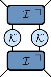
$$ \begin{aligned} \mathcal{K} &= \exp\left[-i b X\right]\\ \mathcal{I} &= \exp\left[-iJ Z_1 Z_2 -i \left(h_1 Z_1 + h_2 Z_2\right)/2\right]. \end{aligned} $$
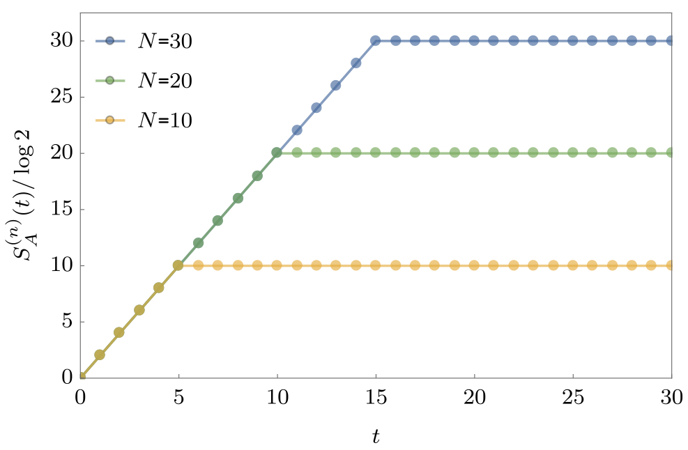
Entanglement Growth for Self-Dual KIM
- Bertini, Kos, Prosen (2019) found that when $|J|=|b|=\pi/4$
$$ \lim_{L\to\infty} S_A =\min(2t-2,N_A)\log 2, $$
- Any $h_j$; initial $Z_j$ product state
Dual unitarity
- Recall KIM has circuit representation
$$ \begin{aligned} \mathcal{K} &= \exp\left[-i b X\right]\\ \mathcal{I} &= \exp\left[-iJ Z_1 Z_2 -i \left(h_1 Z_1 + h_2 Z_2\right)/2\right]. \end{aligned} $$
- At $|J|=|b|=\pi/4$ model is dual unitary
‘KIM’ property
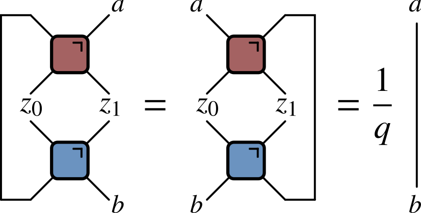
($q=2$ here) Not satisfied by e.g. $\operatorname{SWAP}$
Maps product states to maximally entangled (Bell) states
Product initial states also work for KIM!
Piroli et al (2020) studied more general initial states
Correlation functions
- Infinite temperature correlator $\tr\left[\sigma^\alpha_x(x,t)\sigma^\beta(y,0)\right]$
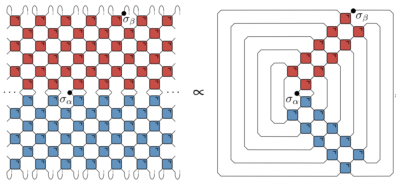
- Bertini, Kos, and Prosen (2019): dual unitarity means correlations vanish inside light cone!
Krajnik-Prosen model
- Classical circuit
$$ \begin{align*} \Phi_{\tau}\left(\mathbf{S}_{1}, \mathbf{S}_{2}\right) &=\frac{1}{\sigma^{2}+\tau^{2}}\left(\sigma^{2} \mathbf{S}_{1}+\tau^{2} \mathbf{S}_{2}+\tau \mathbf{S}_{1} \times \mathbf{S}_{2}, \sigma^{2} \mathbf{S}_{2}+\tau^{2} \mathbf{S}_{1}+\tau \mathbf{S}_{2} \times \mathbf{S}_{1}\right) \\ \mathbf{S}_1^2&=\mathbf{S}_1^2=1\qquad \sigma^{2} =\frac{1}{2}\left(1+\mathbf{S}_{1} \cdot \mathbf{S}_{2}\right) \end{align*} $$
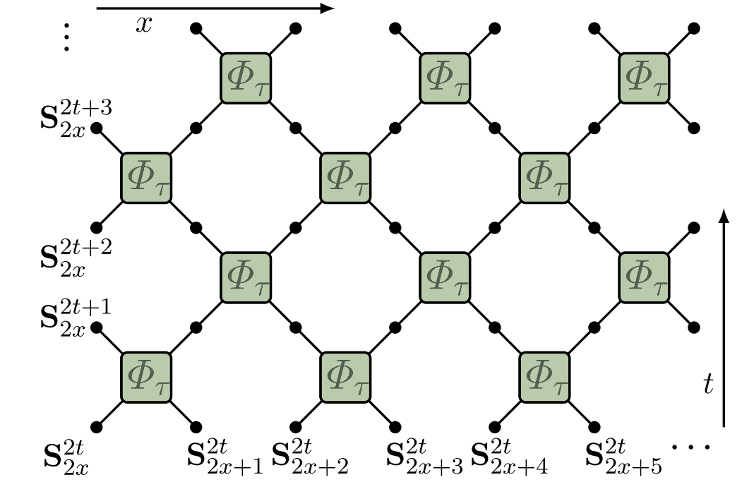
“Space-time duality” of KP model
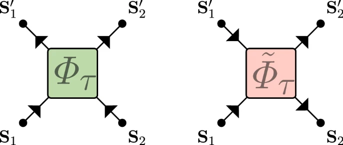
- $\tilde\Phi_\tau$ coincides with $\Phi_\tau$ after flipping
$$ \mathbf{S}_x^t \longrightarrow \tilde{\mathbf{S}}_x^t = (-1)^{x+t+1}\mathbf{S}_x^t $$
Nonzero correlations in the KP model
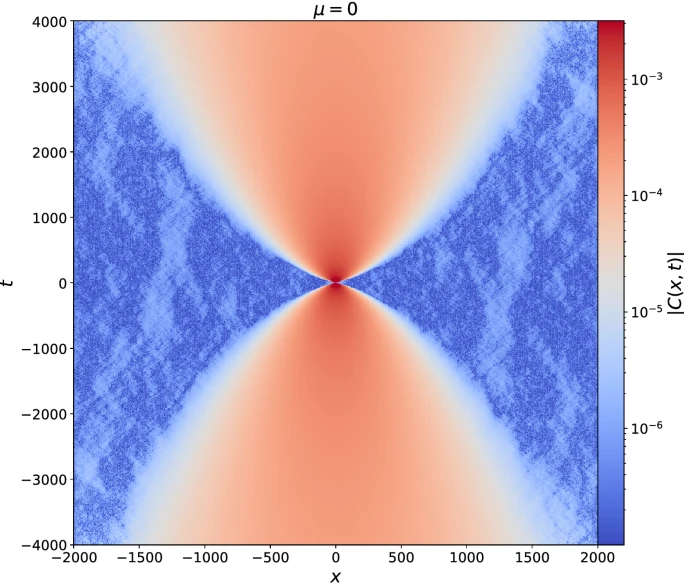
Model is not space-time dual in same sense as dual unitary circuits!
Outline
Cellular automata: elementary, block, reversible, etc.
Space-time duality for CA
Models with continuous state space
Clifford circuits
Conway’s Game of Life
- Any live cell with two or three live neighbours survives
- Any dead cell with three live neighbours becomes a live cell
- All other live cells die in the next generation
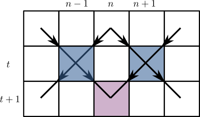
Elementary cellular automata
“Space” is one dimension with cells $x_n=0,1$ $n\in\mathbb{Z}$
Update cells every time step depending on cells in neighborhood
Neighborhood is cell and two neighbors for elementary CA
- Update specified by function
$$ f:\{0,1\}^3\longrightarrow \{0,1\}. $$
$$ x^{t+1}_{n} = f(x^{t}_{n-1},x^{t}_{n},x^{t}_{n+1}) $$
- How many possible functions?
Wolfram’s rules
Domain of $f$ is $2^3=8$ possible values for three cells
$2^8=256$ possible choices for the function $f$
List outputs corresponding to inputs: 111, 110, … 000
| 111 | 110 | 101 | 100 | 011 | 010 | 001 | 000 |
|---|---|---|---|---|---|---|---|
| 0 | 1 | 1 | 0 | 1 | 1 | 1 | 0 |
- Interpret as binary number: this one is Rule 110
Elementary CA
- Many behaviors, from ordered (Rule 18) to chaotic (Rule 30)
- Rule 110 is capable of universal computation!
give each pixel a random Pokemon type, and then battle pixels against their neighbors, updating each pixel with the winning type (using the Pokemon type chart)
— Matt Henderson (@matthen2) July 2, 2022
we quickly see areas of fire > water > grass > fire, electric sweeping over, ground frontiers taking over etc etc pic.twitter.com/BHgQuKRApR
CAs as model physics
Notion of a causal “light cone” (45 degree lines)
Variety of possible behaviors: chaos, periodicity, …
Chaos
- Rapid growth of small differences between two trajectories
- Smallest change: flip one site and monitor $z^t\equiv x^t\oplus y^t$
Chaos phenomenology
No exponential growth (c.f. Lyapunov exponent in continuous systems)
Track number of differences (Hamming distance) between trajectories
Propagating “front” cannot exceed “speed of light”: generally slower
Theory?
No chance of solving the dynamics of any one CA
Looking for generic properties: natural to consider ensembles
- of initial conditions
- of rules
Probabilistic CA
- Choose rules iid for each site and instant
- Cell values are now white noise
Exploring ensemble
Fluctuations of front are larger and average speed $<$ maximum
Interesting variation: choose output $1$ with probability $p$
$p\neq 1/2$ makes dynamics less one-to-one. What happens?
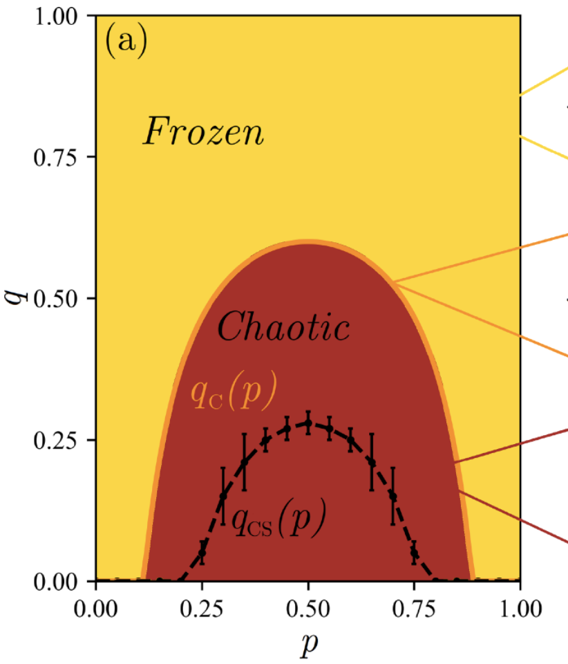
Phase transition
For $0.25\lesssim p\lesssim 0.75$ front propagates to infinity
Outside this region, front dies out
In finite system two copies always merge after exponentially long time
Markov chain on $z^t\equiv x^t\oplus y^t$
- If inputs differ, $z^{t+1}_n=1$ with probability $2p(1-p)$ (Derrida and Stauffer (1986))
- $z^{t+1}_{n}=1$ only if at least one of $z^t_{n\pm 1}=1$
Seek connected cluster of sites occupied with probability $x=2p(1-p)$
This is (site) directed percolation
$x\leq 1/2< x_\text{crit}\sim 0.706$ on square lattice: require NN neighbors
Similar phenomenon in coupled map lattices: “synchronization of extended chaotic systems”
Classical version of MIPT?
Measurements purify state; analogous to non-injective rules in CA
It was a surprise that a mixed state survives finite measurement rate
But… a chaotic front survives non-injective rules (up to a point)
“MIPT” in classical system
Analogous to forced version of transition (Nahum et al. (2021))
Reversibility
No elementary CAs are reversible (bijective)!
Reversibility is undecidable above one spatial dimension
$∃$ reversible constructions
Block cellular automaton

- Partition cells into blocks (Margolus neighborhoods)
- Apply invertible mapping to block
- Alternate overlapping partitions
Spacetime representation
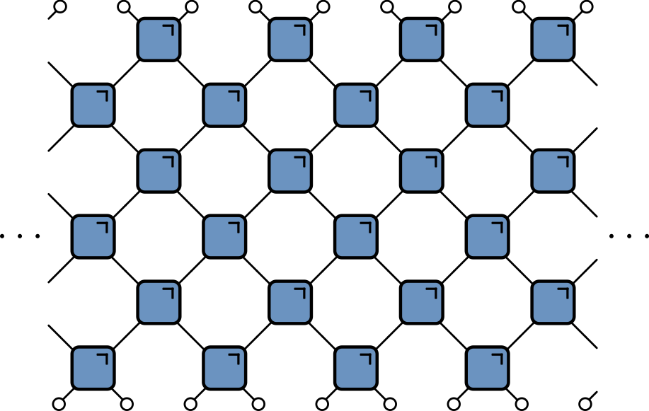
- Blue squares: invertible mapping on states of two sites: 00, 01, 10, 11
given these four jigsaw pieces, there is only one way to fill in the rest of the puzzle. The solution ends up drawing a Sierpinski triangle. Can you see why? pic.twitter.com/OvxVz2oehy
— Matt Henderson (@matthen2) May 25, 2022
24 reversible models
Each block a permutation of 00, 01, 10, 11
$4!=24$ blocks
Order:
- (0123)
- (0132)
- (0213), and so on
Block 2 is the map $(00, 01, 10, 11) ⟶ (00, 10, 01, 11)$ (SWAP)
Reversible CA
Ensemble of block CAs
Results qualitatively similar to chaotic phase of of PCA
No phase transition because all blocks are reversible
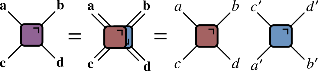
Circuit notation
$$ f:\Sigma\times\Sigma \longrightarrow\Sigma\times\Sigma, \qquad \Sigma=\{0,1\} $$
$$ (c,d) = f(a,b) $$

$$ F_{ab,cd} = \begin{cases} 1 & \text{if } (c,d) = f(a,b) \\ 0 & \text{otherwise} \end{cases} $$
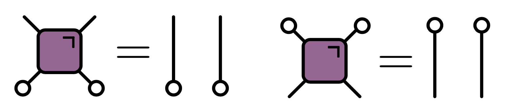
- If $f(\cdot,\cdot)$ is one-to-one:
$$ \sum_{a,b} F_{cd,ab} = \sum_{c,d} F_{cd,ab} = 1 $$
- Circle indicates sum over index
Relaxing 0-1 constraint gives bistochastic matrices
Every bistochastic matrix is a (nonunique) convex combination of permutations (Birkhoff—von Neumann)
Interpret Markov chain as probabilistic BCA
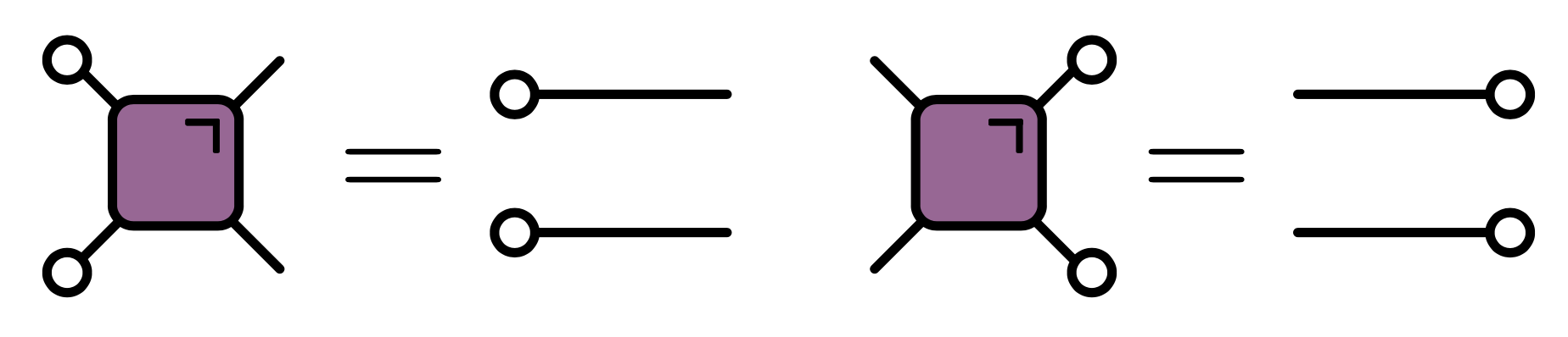
Dual reversibility
- If $(c,d)=f(a,b)$ require bijection $\tilde f$ satisfying $(d,b)=\tilde f(c,a)$
- In terms of $F_{ab,cd}$
$$ \sum_{a,c} F_{cd,ab} = \sum_{b,d} F_{cd,ab} = 1 $$
Equivalent formulation
- Write
$$ \begin{align*} f(a,b)=(f_c(a,b),f_d(a,b))\\ \tilde f(c,a)=(\tilde f_d(c,a),\tilde f_b(c,a)) \end{align*} $$
- Dual reversibility implies that the maps $f_c(a,\cdot)$ and $f_d(\cdot,b)$ are bijections across diagonal
Three state models
Of the 24 reversible blocks for two states, 12 are dual reversible
Three states: Borsi and Pozsgay (2022) find 227 DR models
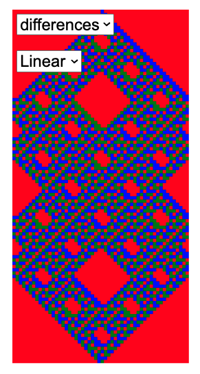
The linear block
$$ (c,d) = f(a,b) = (a + b, a - b), \mod 3 $$
- Original dual unitary circuit from Hosur et al.
- Unusual behavior of recurrence time
- For $L = 2\times 3^m$ have $T_\text{recur}=2L$
- Borsi and Pozsgay prove using Fourier analysis over finite fields
Origin of “fractal” recurrence
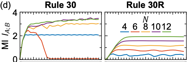
Mutual information
Disjoint regions $A$ and $\bar A$: how much does one tell about the other?
Use mutual information: measure of dependence of random variables
Suggested in this context by Pizzi et al. (2022)
MI defined as $$ I(X;Y) \equiv S(X) + S(Y) - S(X,Y) $$
- $S(X)$ is entropy of $p_X(x)$; marginal distribution of $X$
- $S(Y)$ is entropy of $p_Y(y)$; marginal distribution of $Y$
- $S(X,Y)$ is entropy of joint distribution $p_{(X,Y)}(x,y)$
Vanishes if $p_{(X,Y)}(x,y)=p_X(x)p_Y(y)$
Simple example
- Suppose either $X=Y=1$ or $X=Y=0$, with equal probability
$$ \begin{align*} p_{(X,Y)}(0,0)&=p_{(X,Y)}(1,1)=1/2\\ p_{(X,Y)}(1,0)&=p_{(X,Y)}(0,1)=0 \end{align*} $$
$$ I(X;Y)=S(X) + S(Y) - S(X,Y)= 1+1-1=1 \text{ bit} $$
Toy model (classical reprise)
- Initial distribution factorizes over correlated pairs
- Apply SWAPs
- 1 bit MI for every pair with one member in $A$ and one in $\bar A$
$$ I(A;\bar A) = \min(4\lfloor t/2\rfloor, |A|) \text{ bits} $$
- $|A|$ is (even) number of sites in $A$
Comments
Total entropy conserved (c.f Liouville’s theorem)
Entropy of initial distribution is half max, but entropy $S(A)$ saturates at maximal value (thermalization in time $\sim |A|/2$)
This model is not so special! Any of the dual reversible BCAs behaves exactly the same!
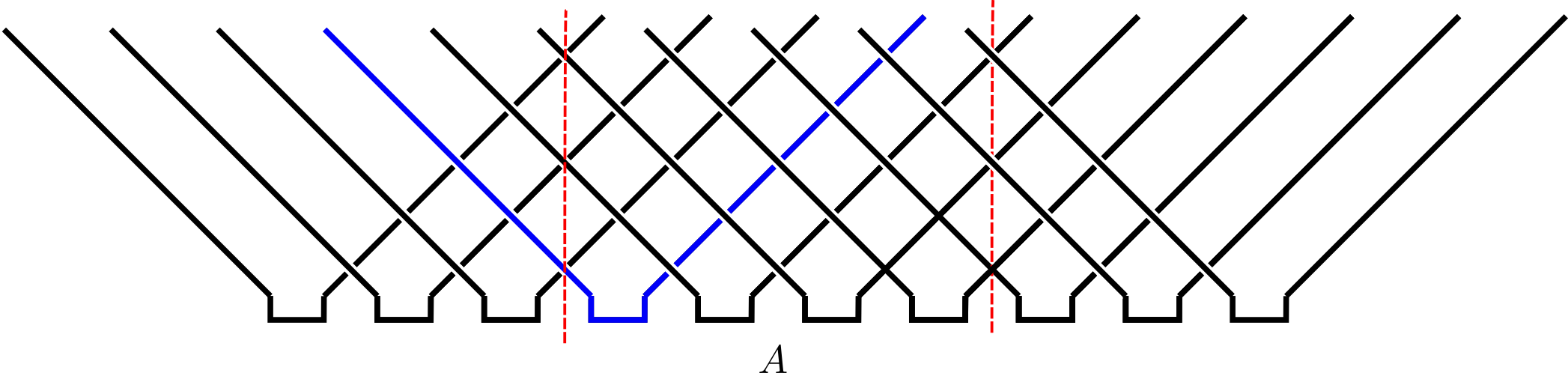
Graphical proof same as for dual unitaries
- $S(A)$ for 8 central sites
- Marginalize over $\bar A$
- After using dual reversibility, result is reversible automaton applied to initial state with $S(A)=6$ bits
Models with continuous state space
$$ f:\Sigma\times\Sigma \longrightarrow\Sigma\times\Sigma $$
Reversible: $f$ must be a bijection, so inverse $f^{-1}$ exists
Probability distribution $p(a,b)$ on two sites is mapped to a distribution $$ p_f(c,d) = |\det Df|^{-1} p(f^{-1}(c,d)), $$ $Df$ is Jacobian matrix
Impose $|Df|=1$ so that uniform (infinite temperature) distribution is preserved
Landau—Lifshitz circuit
- Krajnik and Prosen (2020) studied integrable model
$$ \begin{align*} \Phi_{\tau}\left(\mathbf{S}_{1}, \mathbf{S}_{2}\right) &=\frac{1}{\sigma^{2}+\tau^{2}}\left(\sigma^{2} \mathbf{S}_{1}+\tau^{2} \mathbf{S}_{2}+\tau \mathbf{S}_{1} \times \mathbf{S}_{2}, \sigma^{2} \mathbf{S}_{2}+\tau^{2} \mathbf{S}_{1}+\tau \mathbf{S}_{2} \times \mathbf{S}_{1}\right) \\ \sigma^{2} &:=\frac{1}{2}\left(1+\mathbf{S}_{1} \cdot \mathbf{S}_{2}\right) \end{align*} $$
- Symplectic map on $S^2\times S^2$
Dual reversibility
As before $(d,b) = \tilde f(c,a)$. Require $|D \tilde f|=1$
Discrete case: bijectivity of $\tilde f$ equivalent to existence of diagonal bijections $f_c(a,\cdot):\Sigma_b\longrightarrow \Sigma_c$ and $f_d(\cdot,b):\Sigma_a\longrightarrow \Sigma_d$
Continuous case: additional condition: bijections have unit determinant
- Recall $$ p_f(c,d) = |\det Df|^{-1} p(f^{-1}(c,d)), $$
- Equivalent to $$ p_f(c,d) = \int \delta((c,d)-f(a,b)) p(a,b), d\mu(a) d\mu(b) $$ $$ 1 = \int \delta((c,d)-f(a,b))\, d\mu(a) d\mu(b) $$
- $|D\tilde f|=1$ guarantees that
$$ 1 = \int \delta((d,b)-\tilde f(c,a))\, d\mu(a) d\mu(c) $$
- Not analog of
- Even if $(c,d)=f(a,b)$ and $(d,b)=\tilde f(c,a)$: $$ \delta((c,d)-f(a,b))\neq \delta((d,b)-\tilde f(c,a)) $$
Necessary condition
$$ \delta((c,d)-f(a,b))= \delta((d,b)-\tilde f(c,a)) $$
- Requires diagonal bijections satisfy
$$ |Df_c(a,\cdot)|=1\qquad |Df_d(\cdot,b)|=1 $$
- Not satisfied by Krajnik—Prosen model!
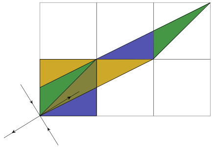
Symplectic dynamics
State space $\Sigma$ is symplectic manifold with symplectic form $\omega$
$f:\Sigma\times\Sigma\longrightarrow\Sigma\times\Sigma$ obeys $f^{*}(\omega_1+\omega_2)=\omega_1+\omega_2$
$\omega$ has (locally) canonical form
$$ \omega = \sum_{i=1}^{n} dx_i\wedge dy_i $$
- $Df$ is symplectic matrix
$$ \begin{align*} Df^T \Omega Df &= \Omega\qquad \Omega \equiv\operatorname{diag}(\omega,\omega)\\ \omega &= \begin{pmatrix} 0 & \mathbb{1}_n \\ -\mathbb{1}_n & 0 \end{pmatrix} \end{align*} $$
Rearranging gives condition on spatial Jacobian $D\tilde f$ $$ D\tilde f^T\operatorname{diag}(\omega,-\omega) D\tilde f = \operatorname{diag}(-\omega,\omega). $$
$\tilde f$ not symplectic but may be made so by composing with pair of maps $\tau_{1,2}$ that reverse signs of $\omega_1$ and $\omega_2$ e.g. $\tau_{1,2}$ $y_i\to -y_i$
$\tau_2\circ \tilde f\circ \tau_1$ is then symplectic
In Krajnik—Prosen model this corresponds to $$ \mathbf{S}_x^t \longrightarrow \tilde{\mathbf{S}}_x^t = (-1)^{x+t+1}\mathbf{S}_x^t $$
Any symplectic map volume preserving in spatial direction
Arnold’s Cat map
- Area preserving (symplectic) linear map on torus
$$ \mathcal{K}:\begin{pmatrix} x \\ y \end{pmatrix}\longrightarrow \begin{pmatrix} a & 1 \\ ab - 1 & b \end{pmatrix} \begin{pmatrix} x \\ y \end{pmatrix}\qquad \mod 1 $$
- Chaotic when one Lyapunov exponent exceeds one for $|a+b|>2$.
- Common choice $a=2$, $b=1$
Spatiotemporal cat
Gutkin and Osipov (2016) define map on $N$ copies of torus
Coupling between sites via
$$ \begin{align*} x_{n}&\longrightarrow x_n \\ y_{n}&\longrightarrow y_n - x_{n-1} - x_{n+1} - V'(x_n) \end{align*}\qquad \mod 1 $$Generated by Hamiltonian (NB $V(x)$ periodic) $$ H_\text{c} = \sum_n \left[x_{n} x_{n+1} + V(x_n)\right] $$
Alternate with cat maps $\mathcal{K}_n$ on each site
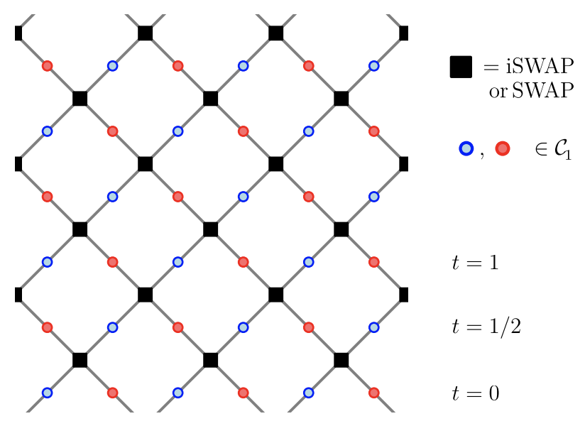
Circuit form
- On neighbouring sites define
$$ \mathcal{I}_{n,n+1}:\qquad\begin{align} x_{n}&\longrightarrow x_n,\qquad x_{n+1}\longrightarrow x_{n+1} \\ y_{n}&\longrightarrow y_n - x_{n+1}-V'(x_n)/2\qquad y_{n+1}\longrightarrow y_{n+1} - x_{n}-V'(x_{n+1})/2,\qquad \mod 1, \end{align} $$
- Satisfies dual reversible property!
Lagrangian pictue
“Momenta” $y_n$ can be eliminated to give two-step (Lagrangian) recurrence for $x_{n,t}$:
$$ [\Delta x]_{n,t} = (a+b-4)x_{n,t} - V'(x_{nt})-m_{n,t} \mod 1 $$winding numbers $m_{n,t}$ chosen to ensure $x_{n,t}$ stays in the unit interval and $\Delta$ is the 2D LaplacianSymmetry between space and time is evident (but not necessary for dual reversibility)
Vary coupling ($V(x)=0$)
$$ H_\text{c} = J\sum_n x_{n} x_{n+1} \qquad J\in \mathbb{Z} $$
$$ \begin{pmatrix} x_n \\ y_n \\ x_{n+1} \\ y_{n+1} \end{pmatrix}\longrightarrow \begin{pmatrix} a & 1 & -J & 0 \\ J^2 + ab - 1 & b & -J(a+b) & -J \\ -J & 0 & a & 1 \\ -J(a+b) & -J & J^2 + ab -1 & b \end{pmatrix}\begin{pmatrix} x_n \\ y_n \\ x_{n+1} \\ y_{n+1} \end{pmatrix} $$
- Off-diagonal blocks have det $J^2$; diagonals $1-J^2$
Symplectic conservation law
Clifford circuits and symplectic CA (Schlingemann et al (2008))
Local space $\mathbb{C}^p$ ($p$ prime): $X$ (“shift”) and $Z$ (“clock”) $$ X\ket{q} = \ket{q+1},\qquad Z\ket{q}=e^{2\pi iq/p}\ket{q} $$
$w(r,k) \equiv X^rZ^k$ satisfy
$$ w(r_1,k_1)w(r_2,k_2) = e^{2\pi i(r_1k_2-r_2k_1)/p}w(r_2,k_2)w(r_1,k_1). $$
- Clifford unitary maps
$w(r,k)\to w(r',k')$$$ U_\text{c} w(r,k)U^\dagger_{c} = e^{i\theta(r,k)}w(r',k') $$
$$ r_1k_2-r_2k_1 = r'_1k'_2-r'_2k'_1, \mod p $$
If
$$ r_1k_2-r_2k_1 = r'_1k'_2-r'_2k'_1, \mod p $$$$\begin{pmatrix} r' \\ k' \end{pmatrix} =\begin{pmatrix} a & b \\ c & d \end{pmatrix}\begin{pmatrix} r \\ k \end{pmatrix},\mod p $$with $ad-bc=1 \mod p$. Matrix $\in\text{Sp}(2,\mathbb{Z}_p)$.For $N$ sites have $w_N(\textbf{r}, \textbf{k})\equiv\prod_{n=1}^N X^{r_n}Z^{k_n}$, and Clifford unitaries on $N$ sites give symplectic matrix $\text{Sp}(2N,\mathbb{Z}_p)$
Circuit made of Clifford unitary blocks can therefore be specified by gates taken from $\text{Sp}(4,\mathbb{Z}_p)$.
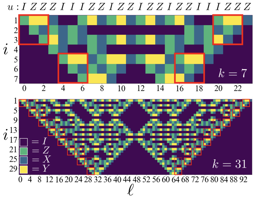
Dual unitary Cliffords circuits
Sommers et al automata
Correlations $\tr\left[\sigma^a_x(x,t)\sigma^b(y,0)\right]$ vanish
OTOC has maximal speed and doesn’t broaden (Claeys and Lamacraft (2020))
MBQC with dual unitary Cliffords
Summary
There is a “useful” notion of space-time duality for classical models
Existing examples: spatiotemporal cat, dual unitary Cliffords
Applications in codes, MBQC?
Thank you!