$$ \nonumber \newcommand{\br}{\mathbf{r}} \newcommand{\bp}{\mathbf{p}} \newcommand{\bk}{\mathbf{k}} \newcommand{\bq}{\mathbf{q}} \newcommand{\bv}{\mathbf{v}} \newcommand{\bx}{\mathbf{x}} \newcommand{\bz}{\mathbf{z}} $$
Hamiltonian Neural Networks
Austen Lamacraft
- Learning Symmetries of Classical Integrable Systems, Roberto Bondesan & AL arXiv:1906.04645
- Hamiltonian Neural Networks, Greydanus et al. arXiv:1906.01563
- Equivariant Hamiltonian Flows, Rezende et al. arXiv:1909.13739
- Hamiltonian Generative Networks, Toth et al. arXiv:1909.13789
- Neural Canonical Transformation with Symplectic Flows, Li et al. arXiv:1910.00024
Outline
- Hamiltonians in physics
- ML background
- Learning dynamics
- Learning canonical transformations
Hamiltonians in Physics
Hamilton’s Equations
- Newton’s law 2nd order in $\mathbb{R}^N$
$$ \begin{aligned} \dot \bq &=\frac{\partial H}{\partial \bp}\\ \dot \bp &=-\frac{\partial H}{\partial \bq} \end{aligned} $$
- 1st order equations in phase space $\mathbb{R}^{2N}$
- Flow along vector field $\bv(\bq,\bp)=(\dot\bq,\dot\bp)$.
- Trajectories are integral curves of $\bv(\bq,\bp)$.
Simple Harmonic Motion
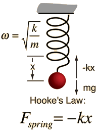
Newton tells us $\ddot x = - \omega^2 x$
General solution $x(t) = A\cos \omega t + B \sin \omega t$
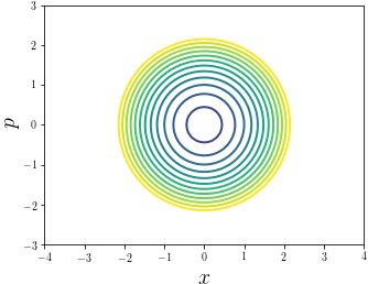
Phase Space
- One 2nd order equation $\longrightarrow$ two 1st order equations
$$ \begin{aligned} \dot x &= p\\ \dot p &= -x \end{aligned} $$
- Observe energy $E=\frac{1}{2}\left[p^2+x^2\right]$ constant
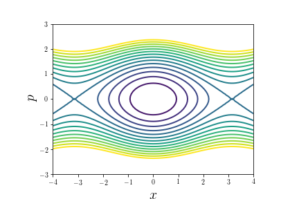
Pendulum
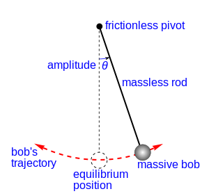
- Newton says
$$ \ddot \theta = -\frac{g}{l}\sin\theta $$
Pendulum in Phase Space
- $\theta\to x$
$$ \begin{aligned} \dot x &= p\\ \dot p &= -\sin x \end{aligned} $$
Hamilton’s equations
- For
$(\mathbf{q}, \mathbf{p})\in\mathbb{R}^{2n}$, Hamiltonian$H:\mathbb{R}^{2n}\to \mathbb{R}$defines dynamics via
$$ \begin{aligned} \dot \bq &= \frac{\partial H}{\partial \bp}\\ \dot \bp &= -\frac{\partial H}{\partial \bq} \end{aligned} $$
- The examples we’ve seen so far have
$$ H(\mathbf{q},\mathbf{p}) = \frac{1}{2}\mathbf{p}^2 + V(\mathbf{q}) $$
- And $H$ is the energy
Geometrical Meaning
- Phase plane velocity
$(\dot\bq,\dot\bp)$perpendicular to $\nabla H$ ($H$ conserved)
$$ (\dot\bq,\dot\bp)\cdot (\nabla_\bq H, \nabla_\bp H) = (\nabla_\bp H,-\nabla_\bq H)\cdot (\nabla_\bq H, \nabla_\bp H) = 0 $$
- Velocity is divergenceless
`$$ \nabla\cdot\bv=\frac{\partial \bv_\bq}{\partial \bq}+\frac{\partial \bv_\bp}{\partial \bp}=\frac{\partial^2 H}{\partial \bq\partial \bp}-\frac{\partial^2 H}{\partial \bp\partial \bq} = 0 $$``
- Flow preserves volume
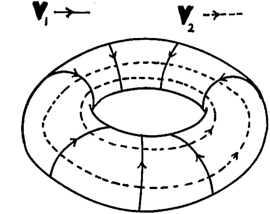
Chaos
- For $N=1$ motion on the contours of $H$ fixes trajectories
- For $N\geq 2$ visualize by taking a Poincaré section
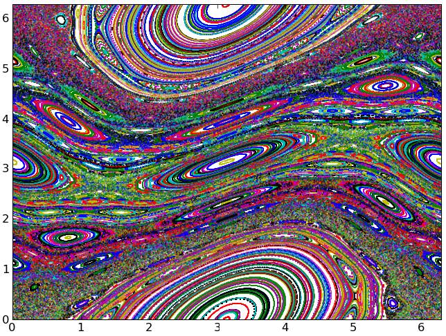
- Generically regions of regular and chaotic motion will occur
Canonical Transformations
Write $x=(\mathbf{q}, \mathbf{p})\in \mathbb{R}^{2N}$
Hamiltonian evolution on $t\in[0,T]$ with $x’=x(T)$, $x=x(0)$
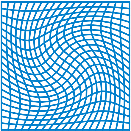
- Example of canonical (symplectic) transformation. What’s special?
Hamilton’s equations
$$ \begin{aligned} \dot \bq &= \frac{\partial H}{\partial \bp}\\ \dot \bp &= -\frac{\partial H}{\partial \bq}\\ \dot{x} &= \Omega \nabla_x H\, ,\quad \Omega = \begin{pmatrix} 0 & \mathbb{1}_n\\ -\mathbb{1}_n & 0 \end{pmatrix} \end{aligned} $$
- Hamilton’s equations $\longrightarrow$ Jacobian $J=\partial x’/\partial x$ satisfies
$$ J^T\Omega J_f = \Omega $$
$J(x)\in\text{Sp}_{2n}(\mathbb{R})$ is member of linear symplectic group
Simplest case $n=1$
$$ J = \begin{pmatrix} a & b \\ c & d \end{pmatrix}\longrightarrow ad-bc=1 $$
- $J\in SL(2,\mathbb{R})$. Rotate / shear / squeeze
$$ J^T\Omega J_f = \Omega $$
Since $\det(J_f) = +1$ $\longrightarrow$ volume is conserved
More: the sum of (signed) areas in each $q_j-p_j$ plane is preserved
- Canonical transformations preserve form of Hamilton’s equations
ML background
Generative Models
Sample from a multivariate distribution
Default approach in physics
$$ P(\{\sigma_i\}) = Z^{-1} \exp\left(-\beta\sum_{i,j}J_{ij}\sigma_i\sigma_j\right) $$
Use MCMC to sample from distribution, calculate expectations, etc.
The Idea (Rezende & Mohamed, 2015)
- Given bijection $\mathbf{f}:\mathbf{x}\mapsto\mathbf{z}$ we have
$$ p_\mathbf{X}(\mathbf{x}) = p_{\mathbf{Z}}(f(\mathbf{x}))\left|\frac{\partial \mathbf{f}}{\partial \mathbf{x}}\right| $$ - Rich $\mathbf{f}$ can yield complex
$p_\mathbf{X}$from simple$p_{\mathbf{Z}}$(e.g. Gaussian) - Parameterize $\mathbf{f}$ with (deep) neural network
- Compose many bijectors
$\mathbf{f}_L\circ \mathbf{f}_{L-1}\cdots \circ \mathbf{f}_1$ - Train by maximizing log-likelihood of data
Application 1: Generation
- Sample: $\mathbf{x}=\mathbf{f}^{-1}(\mathbf{z})$ for $\mathbf{z}\sim p_{\mathbf{Z}}$ (requires invertible $\mathbf{f}$)
- Glow, Diederik P. Kingma, Prafulla Dhariwal, arXiv:1807.03039
Application 2: Density Estimation
- Given $\mathbf{x}$ find $\log p_X(\mathbf{x})$
- Hyunsun Choi & Eric Jang, arXiv:1810.01392
The Challenge
$$ p_\mathbf{X}(\mathbf{x}) = p_{\mathbf{Z}}(f(\mathbf{x}))\left|\frac{\partial \mathbf{f}}{\partial \mathbf{x}}\right| $$
- For $\mathbf{x},\mathbf{x}\in\mathbb{R}^D$ computation of determinant is $O(D^3)$
- Prohibitive for training of large models.
Two Solutions
- Choose $\mathbf{f}_j$ to have tractable jacobian
- Continuous limit
$$ \mathbf{f}(\mathbf{x}) = \mathbf{x}+\epsilon \mathbf{g}(\mathbf{x}) $$ $$ \left|\frac{\partial \mathbf{f}}{\partial \mathbf{x}}\right|\sim 1 +\epsilon \textrm{tr}\left[\frac{\partial \mathbf{g}}{\partial \mathbf{x}}\right] $$
- Let’s look at some examples of the first approach
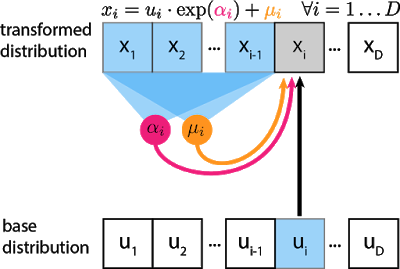
Example 1: Real NVP (Dinh et al, 2016)
- Divide the variables $\mathbf{x}$ into two groups
$x_{1:d}$and$x_{d+1:D}$
$$ \begin{aligned} z_j &= x_j e^{\alpha_j(x_{d+1:D})} + \mu_j(x_{d+1:D}), \qquad j=1,\ldots, d \\ z_j &= x_j \qquad j=d+1,\ldots, D\\ \left|\frac{\partial \mathbf{f}}{\partial \mathbf{x}}\right| &= \prod_{j=1}^d e^{\alpha_i(x_{d+1:D})} \end{aligned} $$
Parameterize scale
$e^{\alpha_j(x_{d+1:D})}$and shift$\mu_j(x_{d+1:D})$by NNCompose many bijections
- Alternating between two sets of variables, or
- Linear orthogonal transformations (c.f. Glow)
Example 2: Autoregressive models
- Exploit chain rule of probability:
$p(\mathbf{x}) = \prod_j p(x_j|x_{1:x_{j-1}})$
$$ x_j = z_j e^{\alpha_j(x_{1:j-1})} + \mu_j(x_{1:j-1}) $$
Learn dynamics
- Hamiltonian Neural Networks, Greydanus et al. arXiv:1906.01563
- Hamiltonian Generative Networks, Toth et al. arXiv:1909.13789
Greydanus et al. arXiv:1906.01563
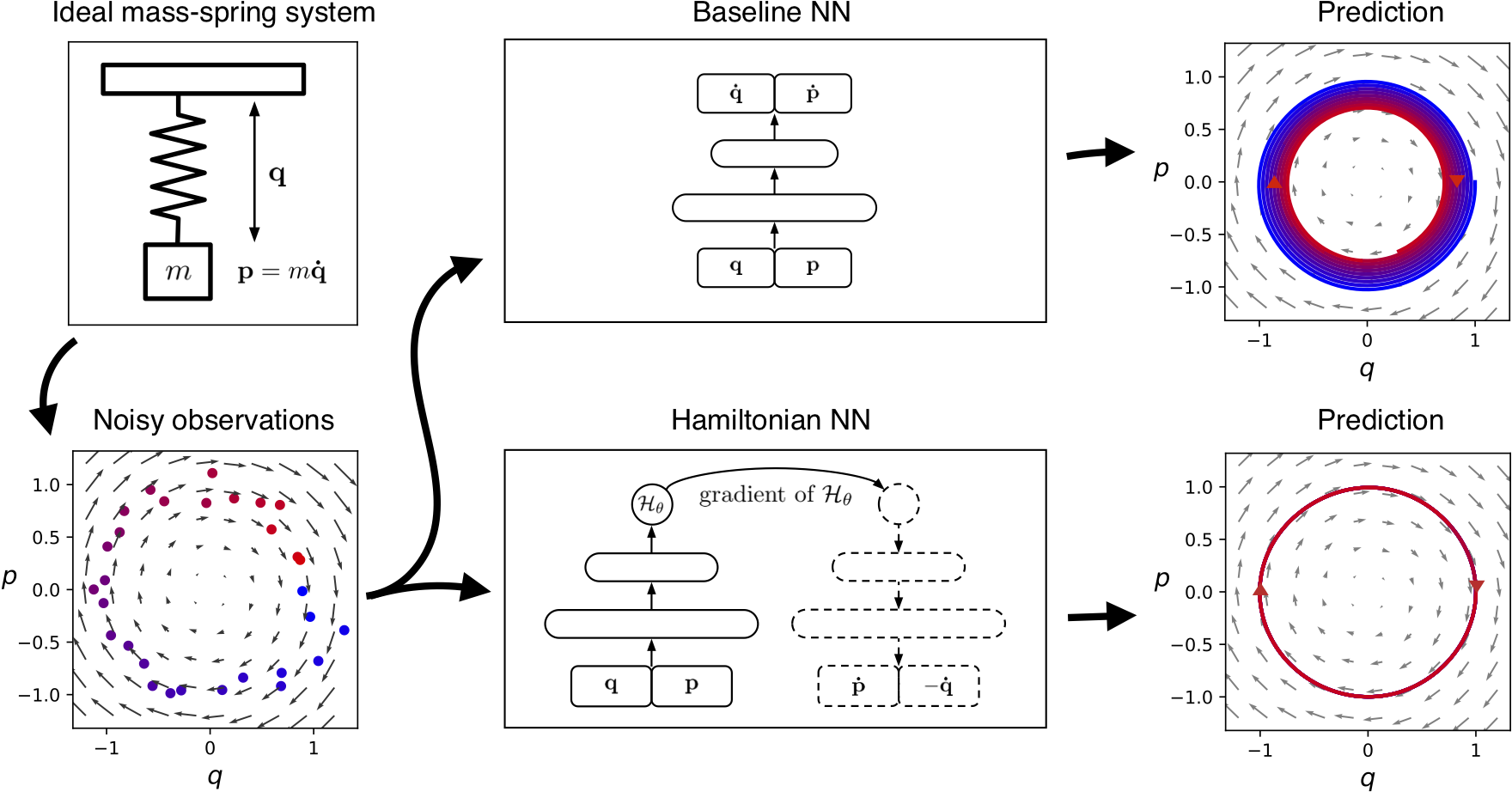
Loss function
$$ \operatorname*{argmin}_\theta \bigg \Vert \frac{d\mathbf{q}}{dt} - \frac{\partial \mathcal{H_{\theta}}}{\partial \mathbf{p}} \bigg \Vert^2 + \bigg \Vert \frac{d\mathbf{p}}{dt} + \frac{\partial \mathcal{H_{\theta}}}{\partial \mathbf{q}} \bigg \Vert^2 $$
- $\mathcal{H_{\theta}}(\bq,\bp)$ parameterized by NN; gradients from AD
Simple tasks
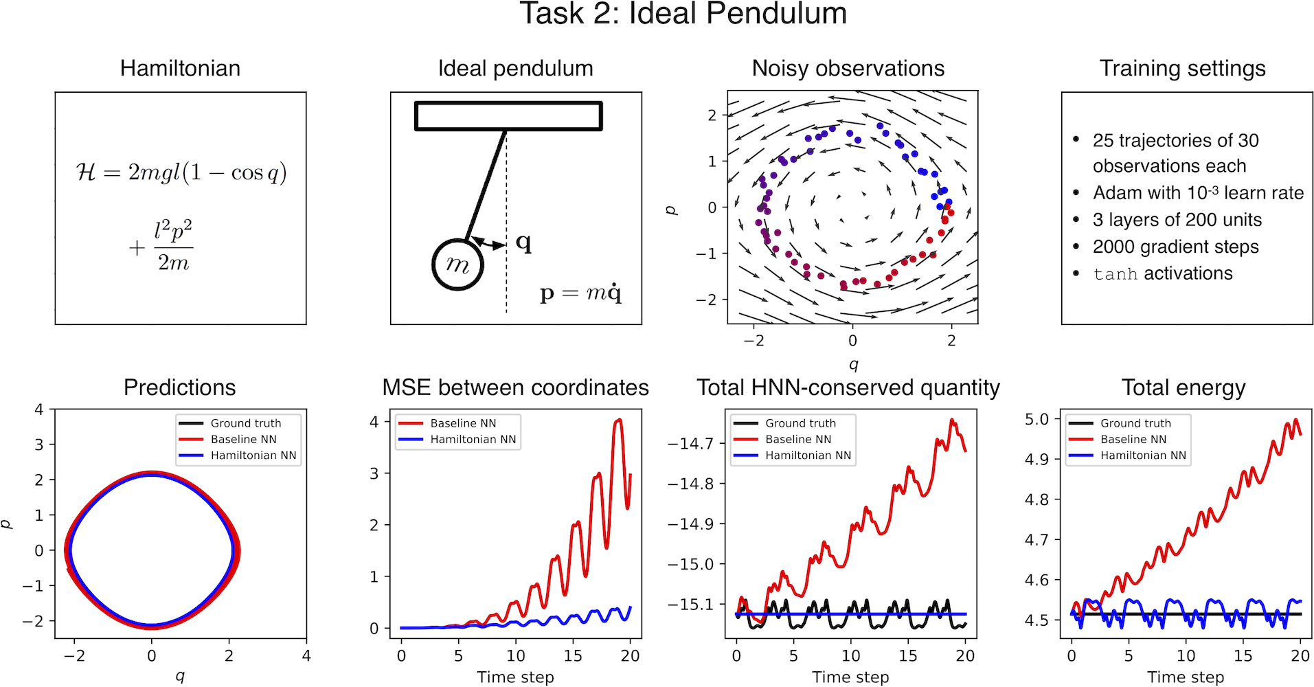
What if you just had an image of the motion?
- Map pairs of images
$\left[\bx_{t}, \bx_{t+1} \right]$to a “latent” phase space $\bz=\left[q_t,p_t\right]$ - Correct dimensionality assumed known
- Toth et al. arXiv:1909.13789 refinement: model the initial point in phase space by an encoder network $\bz\sim q(\cdot|\bx_0,\ldots,\bx_T)$
Neural Canonical Transformations
- Learning Symmetries of Classical Integrable Systems, Roberto Bondesan & AL arXiv:1906.04645
- Neural Canonical Transformation with Symplectic Flows, Li et al. arXiv:1910.00024
How do we choose the right variables?
Generating Functions
- ‘Type 2’ canonical transformation
$$ \mathbf{q}'=\mathbf{q}, \qquad \mathbf{p}'=\mathbf{p}-\nabla F(\mathbf{q}) $$
- c.f. leapfrog, real NVP
$$ z_j = x_j e^{\alpha_j(x_{d+1:D})} + \mu_j(x_{d+1:D}), \qquad j=1,\ldots, d $$
- Differences:
- Only canonical if $\partial_j \mu_k = \partial_k \mu_j$
- No scale (‘NICE’)
Parameterizing shift
- $F(\mathbf{q})\sim \textsf{NN}(\mathbf{q})$ and get $\nabla F(\mathbf{q})$ from autodiff
__Problem__: $O(m^2)$ in training network of $m$ layers.
- Irrotational MLP: $\partial_j \mu_k = \partial_k \mu_j$ if
$$ \mu(\mathbf{q}) = W_1^T\sigma(W_2 \sigma(W_1\mathbf{q})), \qquad W_2 \text{ diagonal} $$
- $\mathbf{q}$ unchanged. More complicated transformations?
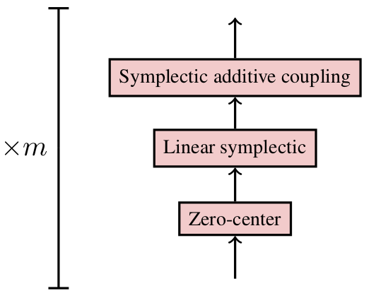
Linear layers
Linear layer to mix $p,q$ so that deeper additive couplings act on all phase space coordinates (c.f. Glow)
To parametrize $S\in \text{Sp}_{2n}(\mathbb{R})$
$$ \begin{aligned} S = NAK= \begin{pmatrix} \mathbf{1} & 0 \\ M & \mathbf{1} \end{pmatrix} \begin{pmatrix} L^\top & 0 \\ 0 & L^{-1} \end{pmatrix} \begin{pmatrix} X & -Y \\ Y & X \end{pmatrix} \, , \end{aligned} $$with$$ \begin{aligned} &M = M^\top \,,\quad &X^\top Y = Y^\top X \, ,\quad X^\top X + Y^\top Y = \mathbf{1}\,. \end{aligned} $$
$$ K = \begin{pmatrix} X & -Y \ Y & X \end{pmatrix} , , $$
- Write in terms of unitary $X + iY$ as product of Householder reflections $$ R_v = \mathbb{1} - 2 \frac{v v^\dagger}{||v||^2}\in {\rm U}_n,, $$ and a diagonal matrix of phases
$$ U = \text{diag}(e^{i\phi_i}),. $$
Zero Center (c.f. Batch Norm)
$$ \begin{aligned} \begin{cases} Q = q - \mu^q + \alpha\ P = p - \mu^p + \beta \end{cases}, , \end{aligned} $$
Training: $\mu$ is batch mean during training
Testing: weighted moving average accumulated during training
Full version of batch norm not canonical
Stack together
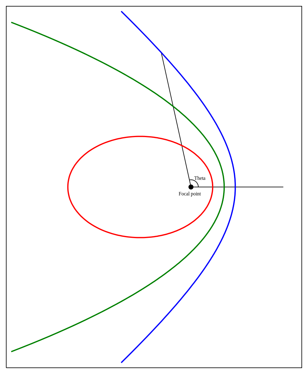
Liouville-Arnold Theorem
Integrable means $N$ conserved phase space functions $I_j$:
Canonical transformations generated by each (as Hamiltonian) commute
Submanifold of phase space at fixed
$\left\{I_{i}\right\}$is $N$-Torus$\mathbb{T}^{N}$
Transformed Hamiltonian
- Transformation $\mathcal{T}$ to action-angle coordinates,
$$ \begin{aligned} \dot{\varphi} = \partial_IK = \text{const.}\,,\quad \dot{I} = -\partial_\varphi K = 0 \end{aligned} $$
- The transformed Hamiltonian $K = H \circ \mathcal{T}$ is independent of the angles
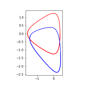
Example: Kepler Hamiltonian
$$ H_{\text{K}} = \tfrac{1}{2}\sum p_i^2 + \frac{k}{r},, \quad r = \sqrt{\sum q_i^2}. $$
$H_\text{K}$ and angular momentum $\mathbf{L}=\mathbf{q}\times\mathbf{p}$ conserved
Additional conserved quantity Laplace–Runge–Lenz vector $$ \mathbf{A} = \mathbf{p}\times\mathbf{L} + k \frac{\mathbf{q}}{r}. $$
Total of 7 conserved quantities. But phase space only 6D!
- Two relations
$$ \begin{aligned} \mathbf{A}\cdot \mathbf{L}&=0\qquad \mathbf{A}^2 &= k^2 + 2H_\text{K} \mathbf{L}^2 \end{aligned} $$
- Trajectories close. This is called superintegrability
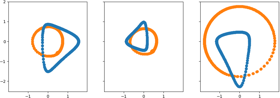
Loss function
- Learn the canonical transformation $T$
$$ T : (\hat{q}, \hat{p}) \mapsto (q, p) ,. $$
$$ \begin{aligned} \ell = \frac{1}{n \tau} \sum_{k=1}^{\tau} || r_{k} - r_{k+1} ||^2\,,\quad r_{k} = \hat{q}(t_k)^2 + \hat{p}(t_k)^2 \,. \end{aligned} $$
- Not canonical: could minimize loss by collapsing the trajectories
Find trajectories from equations of motions (RK)
SGD (Adam)
Shuffle the trajectories at every epoch
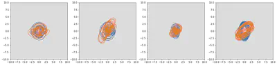
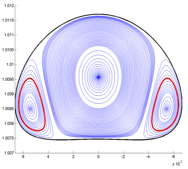
Learning transformation for Kepler Model
Outlook
Continuous canonical transformations (c.f. neural ODE)
Convolutional bijectors, identical particles. etc.
See Neural Canonical Transformation with Symplectic Flows, Li et al. arXiv:1910.00024 for recent developments
Fermi–Pasta–Ulam–Tsingou problem
$$ H = \sum_{i=1}^N \frac{1}{2} [p_i^2 + (q_{i} - q_{i+1})^2] + \frac{\alpha}{3} (q_{i} - q_{i+1})^3 + \frac{\beta}{4} (q_{i} - q_{i+1})^4 $$
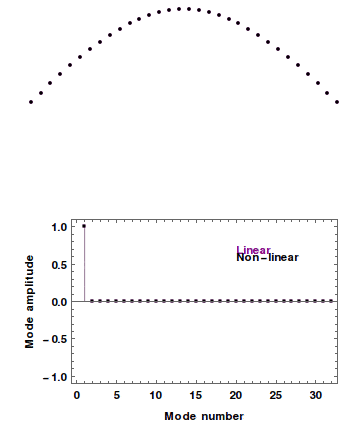
Transform Normal Modes
- $N=5$ sites, 4 nonzero modes