Quantum Circuits
What is a quantum circuit?
- A way to describe operations on quantum state, usually consisting of several qubits (spin 1/2 subsystems)

- $f$ acts on top five qubits, then $g$ acts on lower seven
Possible operations

$H$ (a Hadamard gate) is a single qubit unitary
Also two qubit unitary gates (CNOT here)
Measurements
Why consider circuits?
Model of universal quantum computation
- How to generate an arbitrary quantum state
- One of several options e.g. measurement-based
Example of discrete time, many body dynamics
Unitary circuits
(Mostly) concerned with unitary circuits made from unitary gates
Gate is $n$-qubit unitary $U_{s_1\ldots s_n,s’_1,\ldots, s’_n}$
$$ \sum_{s_1'\ldots s_N'}U_{s_1\ldots s_n,s'_1,\ldots, s'_n} U^\dagger_{s'_1\ldots s'_n,s''_1,\ldots, s''_n}=\delta_{s_1,s_1''}\ldots \delta_{s_N,s_N''} $$
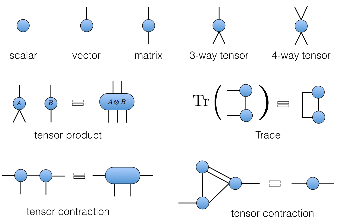
Everything is a tensor
- State of $N$ qubits expressed in product basis
$$ \ket{\Psi} = \sum_{s_{1:N}\in \{0,1\}^N} \Psi_{s_1\ldots s_N}\ket{s_1}_1\ket{s_2}_2\cdots \ket{s_N}_N $$
Write
$\ket{s_1}_1\ket{s_2}_2\cdots \ket{s_N}_N =\ket{s_1\cdots s_N}=\ket{s_{1:N}}$for brevityOperator on $N$ qubits has matrix elements
$$ \mathcal{O}_{s_{1:N},s'_{1:N}} = \bra{s_{1:N}}\mathcal{O}\ket{s'_{1:N}} $$
Graphical notation
Unitary gates: one qubit
Multiplication by a Pauli matrix: $X$, $Y$, or $Z$.
General case $U = a_0\mathbb{1} + \vectorbold{a}\cdot(X,Y,Z)$ with $|a_0|^2+|\vectorbold{a}|^2=1$
Other special cases used in quantum information e.g. Hadamard gate
$$ H = \frac{1}{\sqrt{2}}\begin{pmatrix} 1 & 1 \\ 1 & -1 \end{pmatrix} $$
Two qubits
Usually write in basis $\ket{00}$, $\ket{01}$, $\ket{10}$, $\ket{11}$
Simplest example: SWAP gate
$$ \operatorname{SWAP}=\left[\begin{array}{llll} 1 & 0 & 0 & 0 \\ 0 & 0 & 1 & 0 \\ 0 & 1 & 0 & 0 \\ 0 & 0 & 0 & 1 \end{array}\right] $$Takes product state to product state in computational basis
$$ \operatorname{SWAP}\ket{10} = \ket{01} $$
Square root of SWAP
$$ \sqrt{\operatorname{SWAP}}=\left[\begin{array}{cccc} 1 & 0 & 0 & 0 \\ 0 & \frac{1}{2}(1+i) & \frac{1}{2}(1-i) & 0 \\ 0 & \frac{1}{2}(1-i) & \frac{1}{2}(1+i) & 0 \\ 0 & 0 & 0 & 1 \end{array}\right] $$
- Generates entanglement
$$ \sqrt{\operatorname{SWAP}}\ket{10} = \frac{1}{2}\left[(1+i)\ket{10}+(1-i)\ket{01}\right] $$
Conserves number of 1s and 0s (in fact fully rotationally invariant)
$\sqrt{\operatorname{SWAP}}$ and single qubit unitaries are universal gate set
General two qubit unitary
- Any two-qubit unitary $U\in \mathcal{U(4)}$ can be written
\begin{equation} U = e^{i \phi} (u_+ \otimes u_-) V[J_x, J_y, J_z] (v_- \otimes v_+), \end{equation}
- $u_{\pm}, v_{\pm} \in SU(2)$
\begin{align} V[J_x, J_y, J_z] &= \exp \left[-i\left(J_x \sigma^x \otimes \sigma^x + J_y \sigma^y \otimes \sigma^y+ J_z \sigma^z \otimes \sigma^z\right)\right]\\ &= \begin{bmatrix} e^{-i J_z} \cos(J_-) & 0 & 0 & -i e^{-i J_z \sin(J_-)} \\ 0 & e^{iJ_z} \cos(J_+) & -ie^{i J_z} \sin(J_+) & 0 \\ 0 & -ie^{i J_z} \sin(J_+) & e^{iJ_z} \cos(J_+) & 0 \\ -i e^{-i J_z \sin(J_-)} & 0 & 0 & e^{-i J_z} \cos(J_-) \\ \end{bmatrix} \end{align}
- 16 parameters!
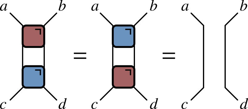
Gate notation
Unitary condition
Time evolution: single qubit gates
Time evolution operator $U=\exp(-iHt)$
If $H=\sum_j h_j$ a sum of single qubit terms
$$ U = \exp(-iHt) = \prod_j \exp(-ih_j) = \prod_j U_j $$ $$ U_j=\mathbb{1}\otimes \ldots \otimes\mathbb{1} \otimes \overbrace{u_j}^{j\text{th factor}} \ldots \otimes\mathbb{1} $$
Two qubit gates
- Simplest example of two qubit interaction is exchange Hamiltonian
$$ \begin{align} h_{12} &= J\left[X\otimes X+Y\otimes Y+Z\otimes Z\right] =J\left[X_1X_2+Y_1Y_2 + Z_1Z_2\right]\\ &=2\operatorname{SWAP} - 1 \end{align} $$ $$ U(J) = \exp(-ih_{12}) = e^{iJ}\left[\cos (2J) \mathbb{1} - i\sin (2J) \operatorname{SWAP}\right] $$
- Special cases
$$ U(\pi/4)=\operatorname{SWAP} $$ $$ U(\pi/8)=\sqrt{\operatorname{SWAP}} $$
$H=\sum_{i,j} h_{i,j}$ a sum of two qubit terms with $[h_{i,j},h_{j,k}]\neq 0$
$U\neq \prod_{i,j} \exp(-ih_{i,j})$. More complicated!
Suzuki–Trotter expansion: decompose $H=H_A + H_B$
$$ U = \exp(-iH) = \left[\exp\left(-\frac{iH}{n}\right)\right]^n \sim \left[e^{-iH_A/n} e^{-iH_B/n}\right]^n $$
Time evolution of chain
$$ H = \sum_j h_{j,j+1} $$ $$ H_A = \sum_j h_{2j, 2j+1}\qquad H_B = \sum_j h_{2j-1, 2j} $$ $$ e^{-iH_A/n}=\prod_j U_{2j,2j+1}\qquad e^{-iH_B/n} = \prod_j U_{2j-1,2j} $$
Floquet theory: kicked Ising model
- Time dependent Hamiltonian with kicks at $t=0,1,2,\ldots$.
$$ \begin{aligned} H_{\text{KIM}}(t) = H_\text{I}[\mathbf{h}] + \sum_{m}\delta(t-n)H_\text{K}\\ H_\text{I}[\mathbf{h}]=\sum_{j=1}^L\left[J Z_j Z_{j+1} + h_j Z_j\right],\qquad H_\text{K} &= b\sum_{j=1}^L X_j, \end{aligned} $$
- “Stroboscopic” form of $U(t)=\mathcal{T}\exp\left[-i\int^t H_{\text{KIM}}(t’) dt’\right]$
$$ \begin{aligned} U(n_+) &= \left[U(1_+)\right]^n,\qquad U(1_-) = K I_\mathbf{h}\\ I_\mathbf{h} &= e^{-iH_\text{I}[\mathbf{h}]}, \qquad K = e^{-iH_\text{K}} \end{aligned} $$
KIM as a circuit

$$ \begin{aligned} \mathcal{K} &= \exp\left[-i b X\right]\\ \mathcal{I} &= \exp\left[-iJ Z_1 Z_2 -i \left(h_1 Z_1 + h_2 Z_2\right)/2\right]. \end{aligned} $$
Locality as a feature of real circuits
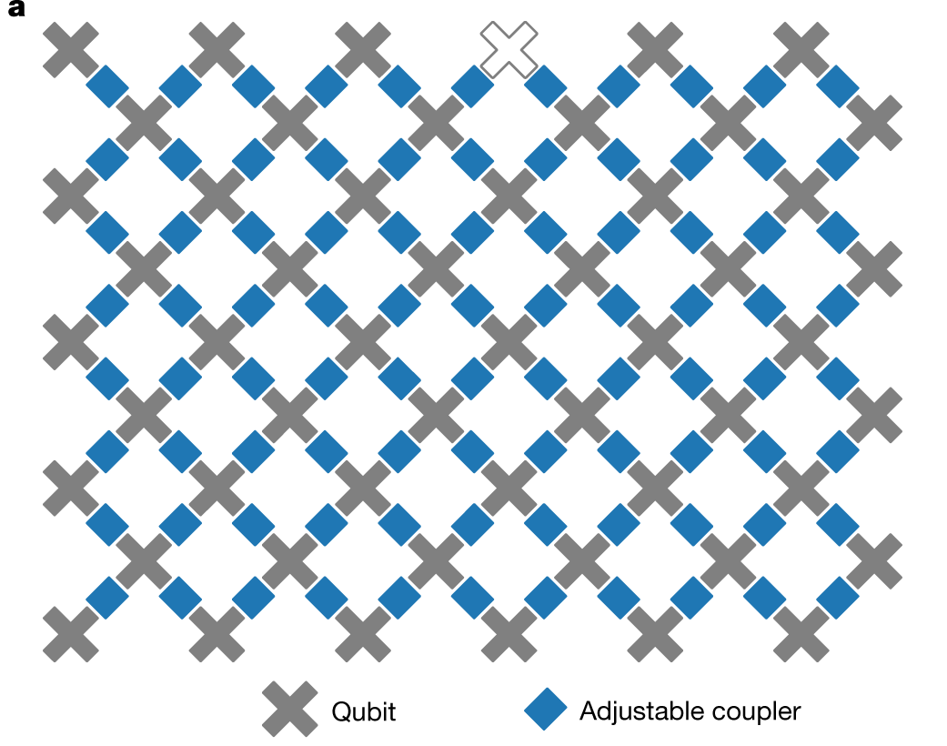
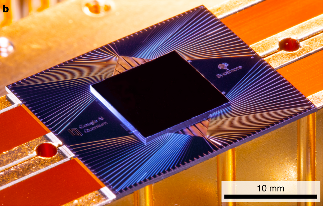
Hype
- Sampling from circuits basis of Google’s “quantum supremacy”

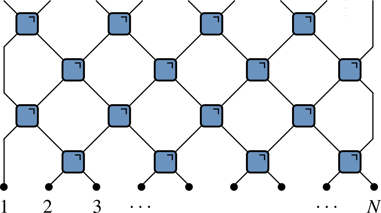
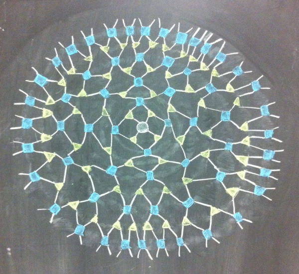
Brickwork unitary circuits
- Have causality built in
- More complicated tensor networks → more complicated spacetimes (black holes, AdS, etc.)
Computational complexity
Normally matrix-vector multiplication is $O(\operatorname{dim}^2)=2^{2N}$
Gates are sparse so $O(\operatorname{dim})=2^{N}$, but still exponentially hard
For low depth $T<N$ move horizontally instead
Expectation values
Evaluate $\bra{\Psi}\mathcal{O}\ket{\Psi}=\bra{\Psi_0}U^\dagger\mathcal{O}U\ket{\Psi_0}$ for local $\mathcal{O}$
If $\Psi_0$ is product state top and bottom indices match
Folded picture
- Recall unitary condtion
After folding lines correspond to two indices / 4 dimensions
Semicircle denotes $\delta_{ab}$
$\bra{\Psi}\mathcal{O}\ket{\Psi}$ in folded picture
- Emergence of “light cone”
Reduced density matrix
$$ \rho_A = \operatorname{tr}_B\left[\ket{\Psi}\bra{\Psi}\right]=\operatorname{tr}_B\left[U\ket{\Psi_0}\bra{\Psi_0}U^\dagger\right] $$
Schmidt decomposition
- In
$\mathcal{H}=\mathcal{H}_A\otimes\mathcal{H}_B$any state$\Psi_{AB}$can be written
$$ \ket{\Psi_{AB}} = \sum_{\alpha=1}^{\min(\operatorname{dim} \mathcal{H}_A, \operatorname{dim} \mathcal{H}_B)} \lambda_\alpha \ket{u_\alpha}_A\otimes\ket{v_\alpha}_B $$
$\ket{u_\alpha}$ and $\ket{v_\alpha}$ orthonormal; $\lambda_\alpha\geq 0$
$\lambda_\alpha$ quantify entanglement between A and B
Apply to reduced density matrix
$$ \begin{align} \rho_A &= \operatorname{tr}_B\left[\ket{\Psi}\bra{\Psi}\right] \\ &= \sum_\alpha \lambda_\alpha^2 \ket{u_\alpha}\bra{u_\alpha} \end{align} $$
- $p_\alpha\equiv \lambda_\alpha^2$ are the eigenvalues of $\rho_A$
Schmidt rank
$\operatorname{rank}=\min(\operatorname{dim} \mathcal{H}_A, \operatorname{dim} \mathcal{H}_B)=2^{\min(2t-2, N_A)}$
Here $t=4$, $N_A=4$
Entanglement entropy
- von Neumann entropy of $\rho_A$
$$ \begin{align} S_A &= -\operatorname{tr}\left[\rho_A\log \rho_A\right]\\ &=-\sum_\alpha p_\alpha \log p_\alpha \end{align} $$
- Maximum value for equal probabilities $p_\alpha = \frac{1}{2^{\min(2t-2, N_A)}}$
$$ S_A \leq \min(2t-2, N_A)\log 2 $$
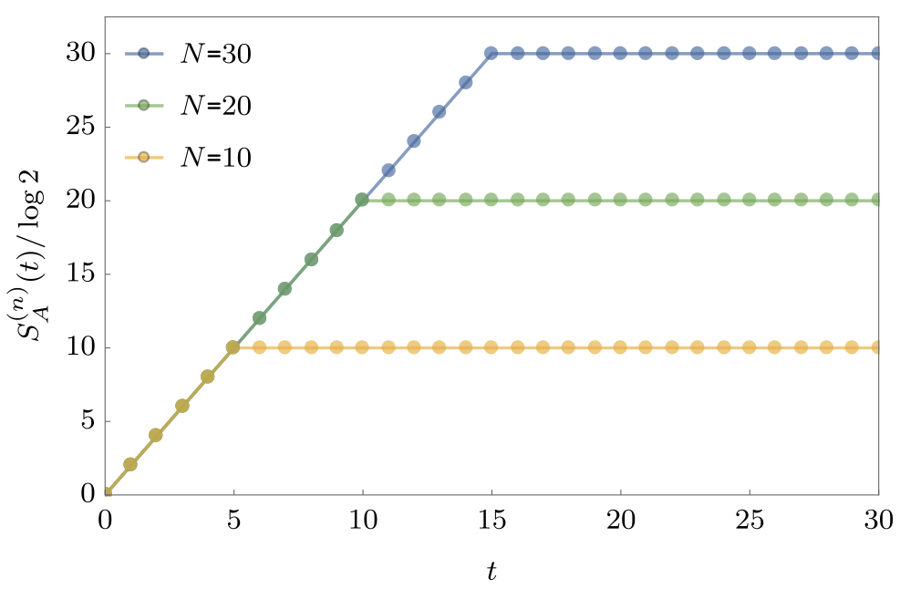
Entanglement Growth for Self-Dual KIM
- Bertini, Kos, Prosen (2019) found that when $|J|=|b|=\pi/4$
$$ \lim_{L\to\infty} S_A =\min(2t-2,N_A)\log 2, $$
- Any $h_j$; initial $Z_j$ product state
Entanglement Spectrum
- Rényi entropies depend on eigenvalues of reduced density matrix
$$ S^{(n)}_A = \frac{1}{1-n}\log \text{tr}\left[\rho^n\right]=\frac{1}{1-n}\sum_\alpha p_\alpha^n $$
- For SDKIM have $2^{\min(2t-2,N_A)}$ non-zero eigenvalues all equal
$$ p_\alpha = \left(\frac{1}{2}\right)^{\min(2t-2,N_A)} $$
Thermalization
After $N_A/2 + 1$ steps, reduced density matrix is $\propto \mathbb{1}$
All expectations (with $A$) take on infinite temperature value
Dual unitarity
- Recall KIM has circuit representation
$$ \begin{aligned} \mathcal{K} &= \exp\left[-i b X\right]\\ \mathcal{I} &= \exp\left[-iJ Z_1 Z_2 -i \left(h_1 Z_1 + h_2 Z_2\right)/2\right]. \end{aligned} $$
- At $|J|=|b|=\pi/4$ has additional property of dual unitarity
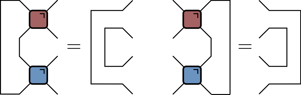
Dual unitarity in folded picture
‘KIM’ property
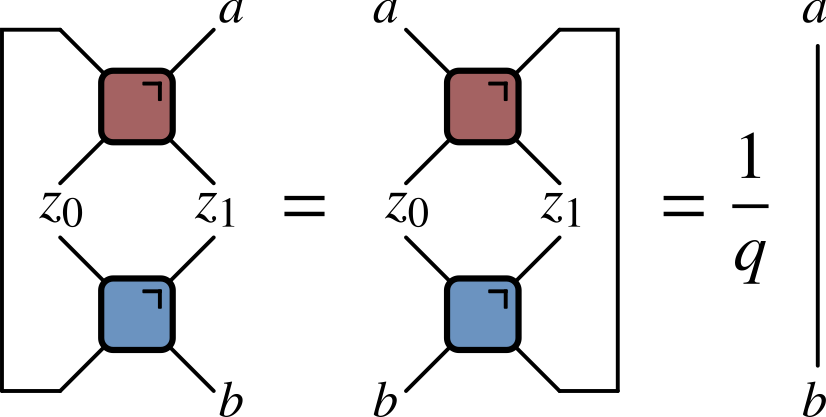
- ($q=2$ here) Not satisfied by e.g. $\operatorname{SWAP}$
‘KIM’ property: folded
$\rho_A$ via dual unitarity + KIM
- RDM is unitary transformation of
$$ \rho_0=\overbrace{\frac{\mathbb{1}}{2}\otimes \frac{\mathbb{1}}{2} \cdots }^{t-1} \otimes\overbrace{|Z_1\rangle\langle Z_1|\otimes |Z_2\rangle\langle Z_2| \cdots }^{N_A-2t+2 } \otimes \overbrace{\frac{\mathbb{1}}{2}\otimes \frac{\mathbb{1}}{2} \cdots }^{t-1} $$
- RDM has $2^{\min(2t-2,N_A)}$ non-zero eigenvalues all equal to $\left(\frac{1}{2}\right)^{\min(2t-2,N_A)}$
Further reading
- Dual unitary circuits were introduced in
- Gopalakrishnan and Lamacraft for kicked Ising
- Bertini, Kos, and Prosen in general
- Piroli et al discuss more general initial conditions