Quantum Circuits II

• austen.uk/slides/quantum-circuits-2

This lecture

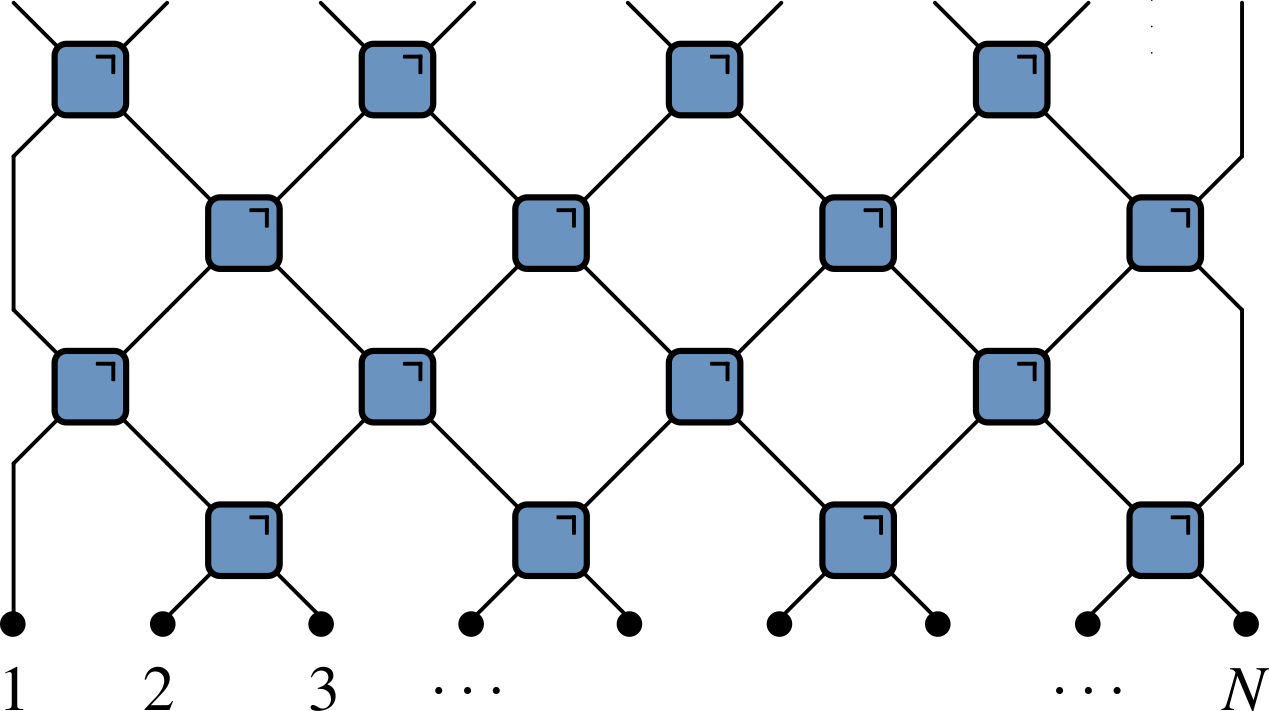
• Correlations near the light cone (see Claeys and Lamacraft for details)

• Operator scrambling and the OTOC

(Infinite temperature) Correlations

$$ c_{\alpha \beta}(x,t) = \langle \sigma_{\alpha}(x,t) \sigma_{\beta}(0,0) \rangle,\qquad \sigma_\alpha(x,t)=U^\dagger(t)\sigma_\alpha(x)U(t) $$

• Vanishes when $|x|>t$ (outside light cone)

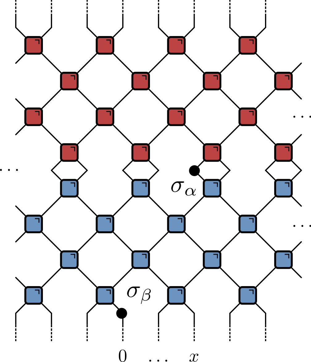
On the light cone

• Using unitarity (only)

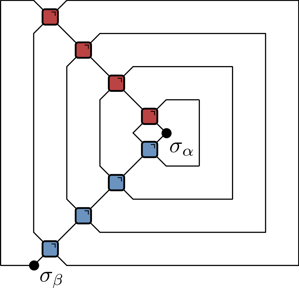
Quantum channel

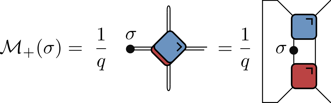
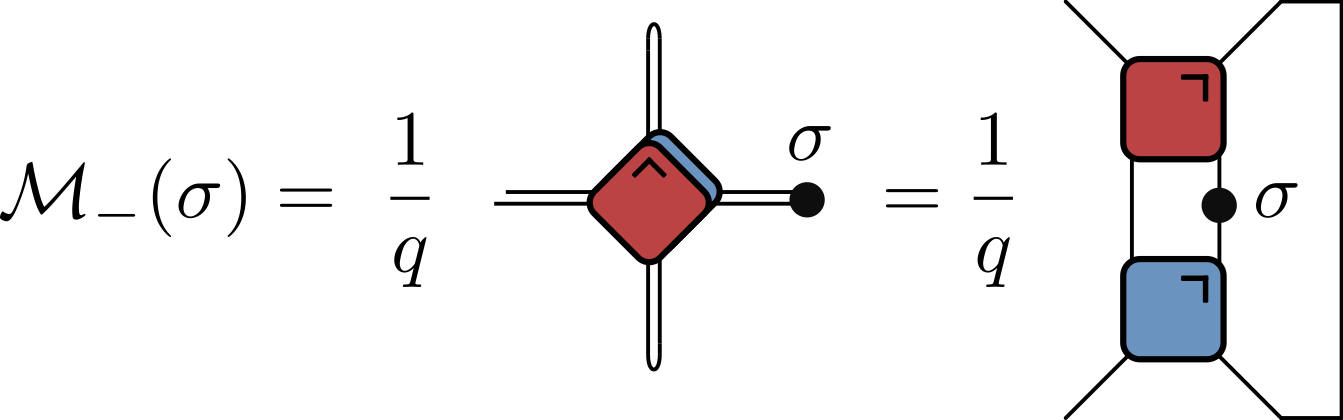
$$ \begin{align}\label{eq:CorrChannels} \langle \sigma_{\alpha}(t,t) \sigma_{\beta}(0,0) \rangle &= \tr \left[\sigma_{\beta}\mathcal{M}_{-}^t(\sigma_{\alpha})\right] / q \\ &= \tr \left[ \sigma_{\alpha}\mathcal{M}_{+}^{t}(\sigma_{\beta})\right] / q \end{align} $$

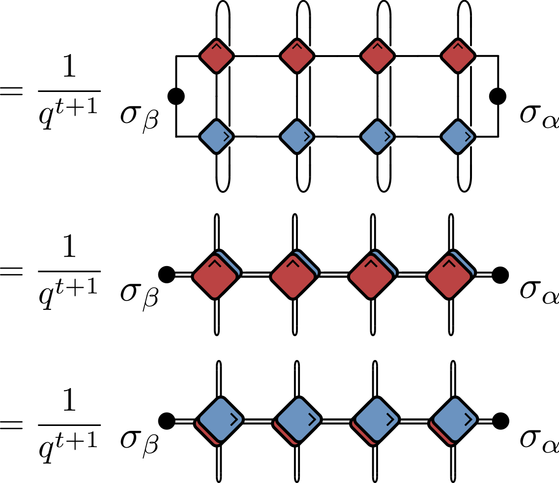
• Calculating correlator involves repeated application of

Typical behaviour of correlations

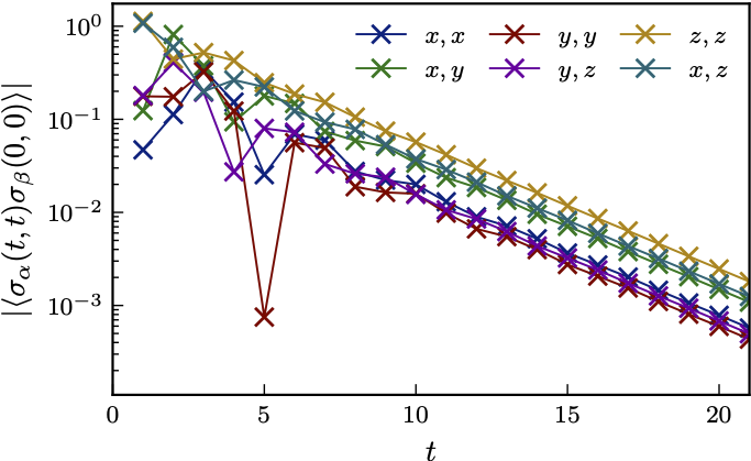
• Surprising that correlations can be found at arbitrary distances!

Correlations for dual unitaries

• Bertini, Kos, and Prosen introduced above formalism for dual unitaries

• Recall light cone $|x|\leq t$ was implied by unitarity

• Dual unitarity implies correlations also vanish for $|x|\geq t$

• Only nonzero correlations are on the light cone

Effect of conservation laws

• $SU(2)$ preserving gate

$$ U_{j,j+1} = \cos\theta \mathbb{1}_{j,j+1} + i\sin\theta \operatorname{P}_{j.j+1} $$

\begin{multline} \mathcal{O} \longrightarrow U^\dagger_{j,j+1}\mathcal{O}U_{j,j+1} = \cos^2\theta \mathcal{O} + \sin^2\theta \operatorname{P}_{j.j+1}\mathcal{O} \operatorname{P}_{j.j+1} \\ -i\sin\theta\cos\theta \left[\operatorname{P}_{j.j+1}, \mathcal{O}\right] \end{multline}

• Generally useful idea: consider random circuit and average

• Take distribution $\theta=\pm \theta_0$ with $p(\theta_0)-p(-\theta_0)\equiv \delta > 0$

Average dynamics

\begin{multline} \overline{U^\dagger_{j,j+1}\mathcal{O}U_{j,j+1}} = \cos^2\theta_0 \, \mathcal{O} + \sin^2\theta_0 \, P_{j.j+1}\mathcal{O} P_{j.j+1} \\ +i\delta \sin\theta_0\cos\theta_0 \left[P_{j.j+1}, \mathcal{O}\right] \end{multline}

• Interpretation:
  • Operators on sites $j$ and $j+1$ switch with probability $\sin^2\theta_0$
  • Asymmetry $\delta$ governs strength of “quantum” dynamics

Continuous time limit

$$ \frac{d\bar{\mathcal{O}}}{dt} = \sum_j \left[iJ \left[P_{j,j+1},\bar{\mathcal{O}}\right]+\left(P_{j,j+1}\bar{\mathcal{O}}P_{j,j+1}-\bar{\mathcal{O}}\right)\right]. $$

\begin{align} i[P,\sigma^a\otimes 1]&=-\epsilon^{abc}\sigma^b\otimes\sigma^c\nonumber\\ i[P,1\otimes \sigma^a]&=\epsilon^{abc}\sigma^b\otimes\sigma^c\nonumber\\ i[P,\sigma^a\otimes \sigma^b]&=\epsilon^{abc}\left(\sigma^c\otimes 1- 1\otimes \sigma^c\right). \label{eq:split-merge} \end{align}

• Sum of first two expressions vanishes by spin conservation

• Describe operator “splitting” ($1\to 2$) and “merging” ($2\to 1$).

Expansion in Pauli basis

$$ Z_j(t)= \sum_{\mu_{1:N}=\{0,1,2,3\}^N} \mathcal{C}_{\mu_{1:N}}(t) \sigma_1^{\mu_1}\otimes\cdots \sigma_N^{\mu_N},\qquad \sigma^\mu = (\mathbb{1},X,Y,Z) $$

• With initial condition

$$ \begin{equation} \mathcal{C}_{\mu_{1:N}}(0)=\begin{cases} 1 & \mu_j=z, \mu_k=0,\forall k\neq j \\ 0 & \text{otherwise}, \end{cases} \end{equation} $$

• Spin correlations $\langle Z_j(t)Z_k(0)\rangle=C_{jk}(t) = \mathcal{C}_{0\cdots \mu_k=z \cdots 0}(t)$

$J=0$: 1 operator sector

• Writing $\mathcal{C}^a_{0\cdots \mu_k=a\cdots 0}\equiv C^a_k$ we have equation of motion

$$ \partial_t C^a_k = C^a_{k+1} + C^a_{k-1} - 2 C^a_k\equiv \Delta_k C^a_k $$

• Diffusion of single $\sigma^a$ ($\Delta_k$ is 1D discrete Laplacian)

Equation of motion

$$ \begin{align} \partial_t \mathcal{C}_{\mu_{1:N}} = \sum_j \left[J\epsilon_{\alpha\beta \mu_j \mu_{j+1}} \mathcal{C}_{\mu_1\cdots \alpha\beta \cdots \mu_N} + \mathcal{C}_{\mu_1\cdots \mu_{j+1}\mu_j \cdots \mu_N} - \mathcal{C}_{\mu_1\cdots \mu_{j}\mu_{j+1} \cdots \mu_N}\right]. \end{align} $$

• See Claeys, Lamacraft, and Herzog-Arbeitman for more

Operator spreading

• Correlations (typically) decay exponentially

• Doesn’t mean that operator dynamics is trivial!

• What can we say about $\sigma_\alpha(x,t)=U^\dagger(t)\sigma_\alpha(x) U(t)$ generally?

$$ Z_j(t)= \sum_{\mu_{1:N}=\{0,1,2,3\}^N} \mathcal{C}_{\mu_{1:N}}(t) \sigma_1^{\mu_1}\otimes\cdots \sigma_N^{\mu_N},\qquad \sigma^\mu = (\mathbb{1},X,Y,Z) $$

• As time progresses two things (tend to) increase

  • Number of non-identity sites (operator spreading)
  • Number of different contributions (operator entanglement)

• How to quantify these?

  • Operator spreading defines “butterfly velocity”
  • Clifford gates lead to operator spreading but no entanglement

Out of time order correlator

$$ \operatorname{OTOC}_{jk}(t) =\langle Z_j(t)Z_k(0)Z_j(t)Z_k(0)\rangle $$

$$ Z_j(t)= \sum_{\mu_{1:N}=\{0,1,2,3\}^N} \mathcal{C}_{\mu_{1:N}}(t) \sigma_1^{\mu_1}\otimes\cdots \sigma_N^{\mu_N} $$

$$ \operatorname{OTOC}_{jk}(t)\propto \sum_{\mu_{1:N}}\mathcal{C}_{\mu_{1:N}}^2(t)\left[\delta_{\mu_k,0}+\delta_{\mu_k,3}-\delta_{\mu_k,1}-\delta_{\mu_k,2}\right] $$

• $\operatorname{OTOC}_{jk}(t)\neq 1$ when operator $Z_j(t)$ spreads from site $j$ to site $k$

• Involves $\mathcal{C}_{\mu_{1:N}}^2(t)$ so survives averaging

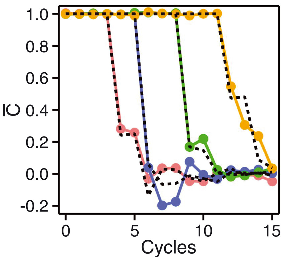
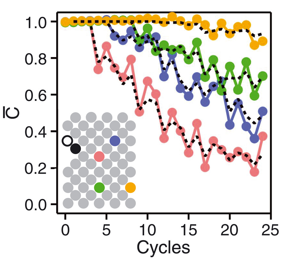
Google’s OTOC experiment

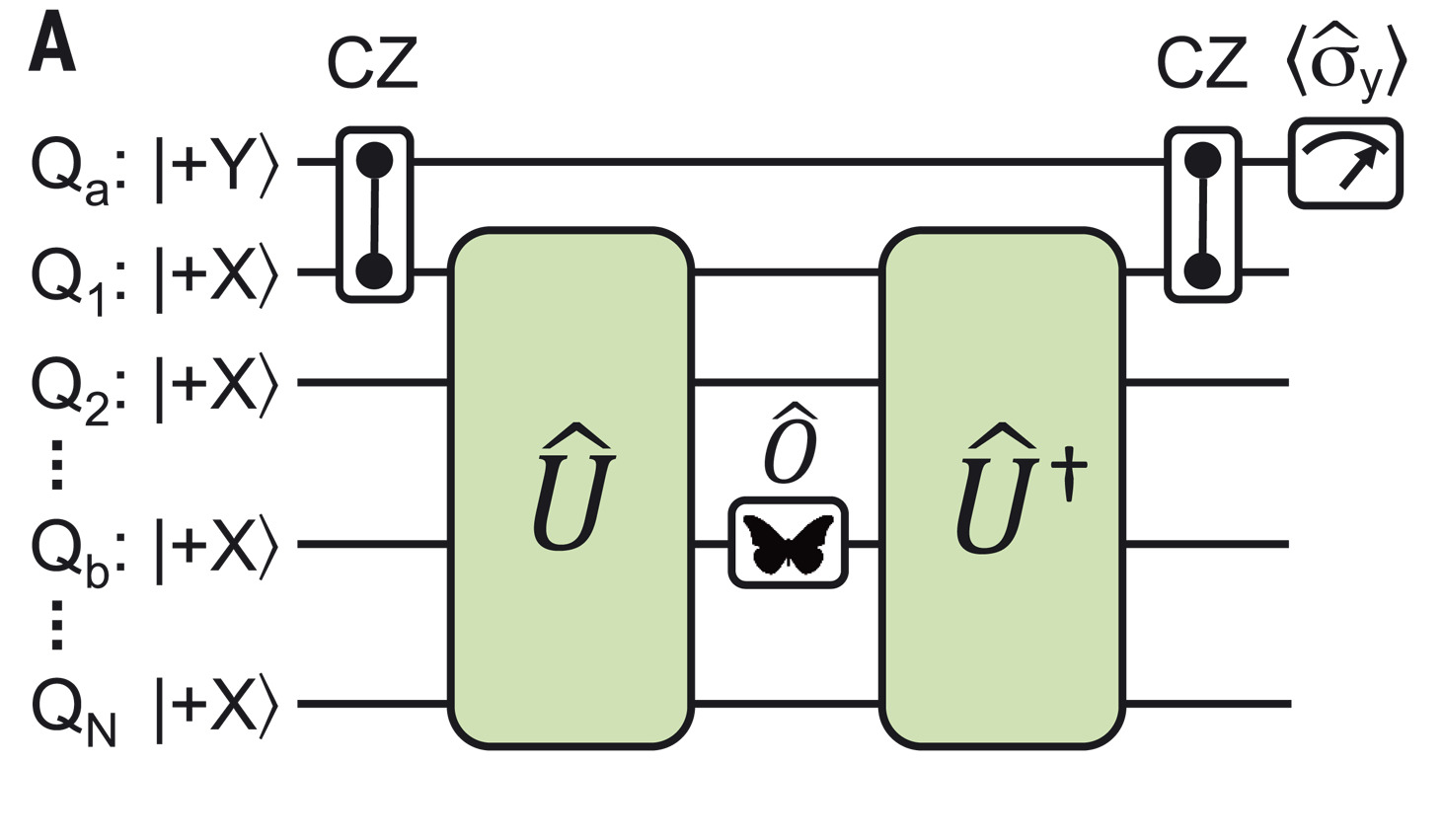
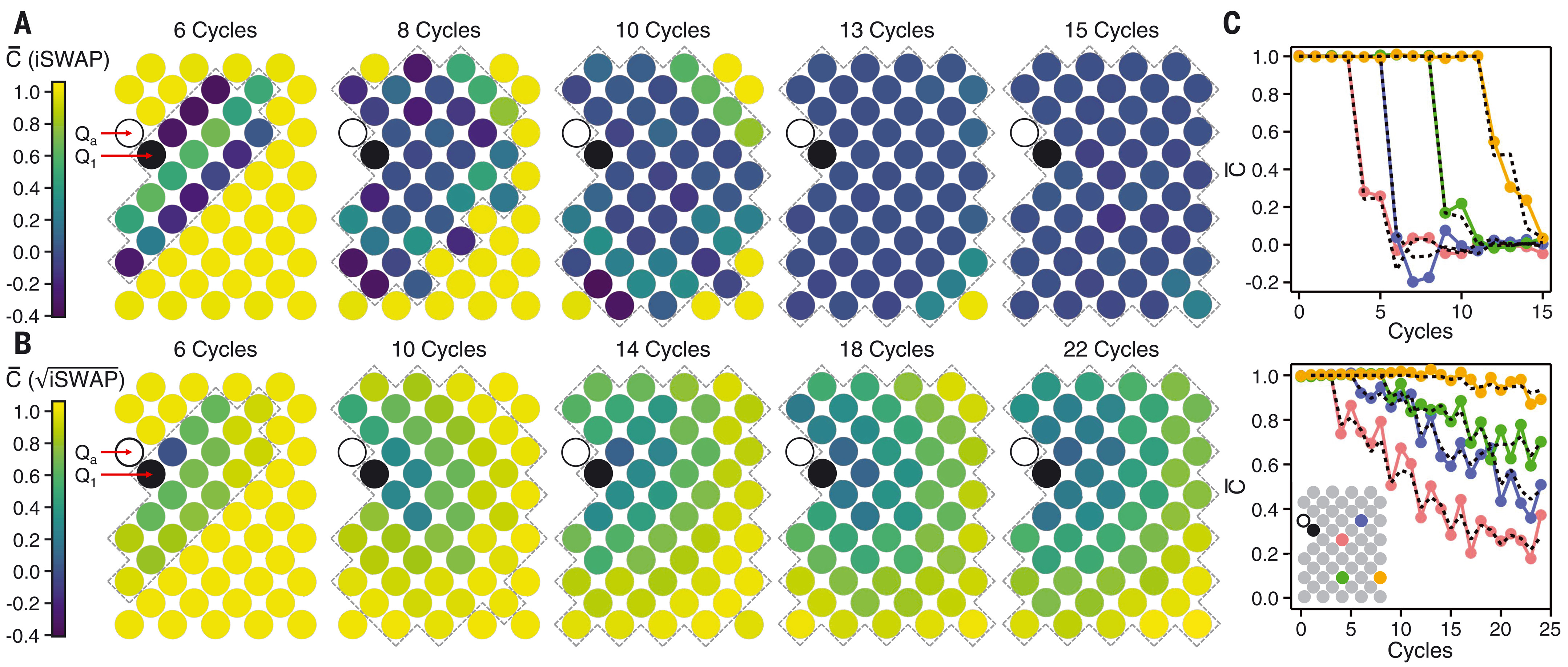
• $i\operatorname{SWAP}$: sharp OTOC front

• $\sqrt{i\operatorname{SWAP}}$: broadened OTOC front

$\overline{\operatorname{OTOC}}$: stochastic model

• See Google’s OTOC experiment (supplementary material)

• Continuous time version in Rowlands and Lamacraft

• Main idea: OTOC extracted from

$$ \hat{\mathcal{O}}^{(2)}(t)=\overline{\hat{O}(t) \otimes \hat{O}(t)} \equiv \overline{\hat{O}(t)^{\otimes 2}} $$

$$ \hat{\mathcal{O}}^{(2)}(t)=\overline{\hat{O}(t) \otimes \hat{O}(t)} \equiv \overline{\hat{O}(t)^{\otimes 2}} $$

• Invariant subspace that survives averaging built from $\mathsf{O} \equiv\mathbb{1}\otimes\mathbb{1}$ and $\mathsf{1}\equiv\frac{1}{3}\left[X\otimes X + Y\otimes Y+ Z\otimes Z\right]$ on each site

• Basis: $\mathsf{S}_{1:N}\equiv\mathsf{S}_1\otimes \mathsf{S}_2\otimes\cdots \mathsf{S}_N$, with $\mathsf{S}_j=0,1$

$$ \hat{\mathcal{O}}^{(2)}(t) = \sum_{\mathsf{S}_{1:N}\in\{\mathsf{0},\mathsf{1}\}^N} P_{\mathsf{S}_{1:N}}\mathsf{S}_{1:N} $$

$$ \hat{\mathcal{O}}^{(2)}(t) = \sum_{\mathsf{S}_{1:N}\in\{\mathsf{0},\mathsf{1}\}^N} P_{\mathsf{S}_{1:N}}\mathsf{S}_{1:N} $$

• (Average of) gate provides update rule for $P_{\mathsf{S}_{1:N}}$ $$ P_{\mathsf{S}_{1:N}}(t+1) = \sum_{\mathsf{S}'_j, \mathsf{S}'_k} P_{\mathsf{S}_1\cdots \mathsf{S}_j \mathsf{S}'_{j+1}\cdots \mathsf{S}'_N}(t)\Omega_{\mathsf{S}'_j \mathsf{S}'_k,\mathsf{S}_j \mathsf{S}_k} $$ $$ \begin{gathered} \Omega=\left(\begin{array}{cccc} 1 & 0 & 0 & 0 \\ 0 & 1-a-b & a & b \\ 0 & a & 1-a-b & b \\ 0 & \frac{b}{3} & \frac{b}{3} & \left(1-\frac{2}{3} b\right) \end{array}\right) \\ a=\frac{1}{3}\left(2 \sin ^{2} \theta+\sin ^{4} \theta\right) \qquad b=\frac{1}{3}\left(\frac{1}{2} \sin ^{2} 2 \theta+2\left(\sin ^{2} \theta+\cos ^{2} \theta\right)\right) \end{gathered} $$
• $\theta=\pi/2$ for $i\operatorname{SWAP}$, $\theta=\pi/4$ for $\sqrt{i\operatorname{SWAP}}$

Markov process

$$ \begin{gathered} \Omega=\left(\begin{array}{cccc} 1 & 0 & 0 & 0 \\ 0 & 1-a-b & a & b \\ 0 & a & 1-a-b & b \\ 0 & \frac{b}{3} & \frac{b}{3} & \left(1-\frac{2}{3} b\right) \end{array}\right) \\ \end{gathered} $$

• Rows sum to one: Stochastic matrix

• Possible transitions

$$\require{extpfeil} \Newextarrow{\xleftrightharpoon}{5,10}{0x21CB} \mathsf{10} \xleftrightharpoon[a]{a} \mathsf{01} \qquad \mathsf{11} \xleftrightharpoon[b/3]{b} \mathsf{10},\mathsf{01} $$

• $\mathsf{00}$ is “inert”

Fredrickson–Andersen model

• Stationary state: independent sites with $p_1=3/4$, $p_0=1/4$

Butterfly velocity

• Front propagation characterised by finite velocity $v_\text{B}$

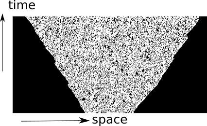
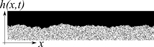
Front broadening

• Front broadens unless $v_\text{B}$ maximal as for $i\operatorname{SWAP}$

• Diffusive in 1D $\propto \sqrt{t}$

• KPZ dynamics in 2D

• See Nahum, Vijay, and Haah for much more

Classical simulation?

• Efficient simulation of averaged OTOC dynamics via Monte Carlo

• Appearance of Markov process a little surprising

OTOC fluctuations

• Circuit-to-circuit fluctuations of OTOC from

$$ \hat{\mathcal{O}}^{(4)}(t)=\overline{\hat{O}(t) \otimes \hat{O}(t) \otimes \hat{O}(t) \otimes \hat{O}(t)} \equiv \overline{\hat{O}(t)^{\otimes 4}} $$

• Go through same procedure of identifying invariant states

• Evolution of average now involves negative matrix elements

• Leads to sign problem in Monte Carlo simulation

• Same problem for $\overline{\operatorname{OTOC}}$ in models with number conservation (Rowlands and Lamacraft)