$$ \nonumber \newcommand{\br}{\mathbf{r}} \newcommand{\bR}{\mathbf{R}} \newcommand{\bp}{\mathbf{p}} \newcommand{\bk}{\mathbf{k}} \newcommand{\bq}{\mathbf{q}} \newcommand{\bv}{\mathbf{v}} \newcommand{\bx}{\mathbf{x}} \newcommand{\bz}{\mathbf{z}} \DeclareMathOperator*{\E}{\mathbb{E}} $$

Quantum Ground States from Reinforcement Learning

Work with Ariel Barr and Willem Gispen

Schrödinger Equation: 1 Particle

• Schrödinger picture: basic object is wavefunction $\psi(\br)$

$$ \overbrace{\left[-\frac{\nabla^2}{2m}+V(\br_i)\right]}^{\equiv H\text{, Hamiltonian}}\psi(\br) = E\psi(\br) $$

• Discretize on real-space grid $L\times L\times L$

Schrödinger Equation: N Particles

• Wavefunction now has $N$ variables: $\Psi(\br_1,\ldots \br_N)$

$$ \overbrace{\left[\sum_i\left(-\frac{\nabla_i^2}{2m_i}+V(\br_i)\right)+\sum_{i<j}U(\br_i-\br_j)\right]}^{\equiv H}\Psi(\br_1,\ldots \br_N) = E\Psi(\br_1,\ldots \br_N) $$

• Requires grid in $3N$ dimensions of $L^{3N}$ points!
• Atoms / molecules are hard; matter ($N\sim N_\text{A}$) is impossible!

Variational Principle

• For approximate $\Psi$ can upper bound ground state $E_0$

$$ \begin{align} E_0 &\leq \inf_{\lVert\Psi\rVert=1} \langle \Psi\lvert H\rvert\Psi\rangle\\ \langle \Psi\lvert H\rvert\Psi\rangle &= \int d\br_1\cdots d\br_N \Psi^*(\br_1,\ldots,\br_N)\left[H \Psi\right](\br_1,\ldots,\br_N) \end{align} $$

Challenges

1. Form of $\Psi$
2. Expectation evaluation
3. Optimization

Form of $\Psi$ (‘Feature Engineering’)

Wavefunctions of restricted form

• Factorized, leading to Hartree–Fock method

$$ \Psi(\br_1,\ldots,\br_N)=\psi_1(\br_1)\ldots \psi_N(\br_N). $$

• Jastrow factors include pair correlations

$$ \Psi(\br_1,\ldots,\br_N)\to \Psi(\br_1,\ldots,\br_N)\exp\left(\sum_{i<j}\phi(\br_i-\br_j)\right) $$

• Many more…

Expectation evaluation

$|\Psi(\br_1,\ldots,\br_N)|^2$ a probability distribution, so evaluate

$$ \frac{\langle \Psi\lvert H\rvert\Psi\rangle}{\langle\Psi \vert\Psi\rangle} =\int d\bR\,|\Psi(\bR)|^2\frac{\left[H \Psi\right](\bR)}{\Psi(\bR)} $$

by Monte Carlo sampling. This is Variational Monte Carlo (VMC)

Neural Approaches

$\Psi(\bR)\sim \textsf{NN}(\bR)$ and optimize!

• Carleo and Troyer (2017): lattice models (more later)

• many more…

• Pfau et al. (2019): Fermi Net

TL;DR

• $\exists$ other formulations of QM including Feynman’s path integral

• Let’s learn the path integral instead!

Outline

• The path integral
• Quantum mechanics and optimal control
• Learning the ground state process
• First experiments
• Next directions

Path integral

• Solution of time-dependent Schrödinger equation

$$ \begin{align} i\frac{\partial \psi}{\partial t} &= H\psi\\ \psi(\br_2,t_2) &= \int d\br_1 \mathcal{K}(\br_2,t_2;\br_1,t_1)\psi(\br_1,t_1),\\ \mathcal{K}(\br_2,t_2;\br_1,t_1) &= \int_{\br(t_1)=\br_1 \atop \br(t_2)=\br_2} \mathcal{D}\br(t)\exp\left(i\int_{t'}^t L(\br(t),\dot{\br})\right) \end{align} $$

• $L(\br,\bv) = \frac{1}{2}\bv^2 - V(\br)$ is the classical Lagrangian

My machines came from too far away

Trouble with Feynman?

• “Integration over paths” has never been defined

• Kac (1949) found a workaround for heat-type equations

\begin{align} \frac{\partial\psi(\br,t)}{\partial t} = \left[\frac{\nabla^2}{2}-V(\br_i)\right]\psi(\br,t) \end{align}

• “Imaginary time” Schrödinger. Exponent in PI becomes real

$$ \exp\left(-\int_{t’}^t \left[\frac{1}{2}\dot\br^2 + V(\br)\right]\right) $$

Feynman–Kac (FK) Formula

…expresses $\psi(\br,t)$ as expectation…

$$ \psi(\br_2,t_2) = \E_{\br(t)}\left[\exp\left(-\int_{t_1}^{t_2}V(\br(t))dt\right)\psi(\br(t_1),t_1)\right] $$

Ground State from PI

• For $t\to\infty$ only ground state contributes

• Spectral representation in terms of $H\varphi_n = E_n\varphi_n$

\begin{align} K(\br_2,t_2;\br_1,t_1) &= \sum_n \varphi_n(\br_2)\varphi^*_n(\br_1)e^{-E_n(t_2-t_1)}\\ &\longrightarrow \varphi_0(\br_2)\varphi^*_0(\br_1)e^{-E_0(t_2-t_1)} \qquad \text{ as } t_2-t_1\to\infty. \end{align}

Bosons and Fermions

• For identical particles $|\Psi(\br_1,\ldots,\br_N)|^2$ permutation invariant

• $\Psi(\br_1,\ldots,\br_N)$ completely symmetric (Bosons) or antisymmetric (Fermions)

• $t\to\infty$ limit picks out nodeless (bosonic) ground states

Path integral Monte Carlo

The Path Measure

• Relative weight of FK paths given by Radon-Nikodym derivative

$$ \frac{d\mathbb{P}_\text{FK}}{d\mathbb{P}_\text{B}} = \mathcal{N}\exp\left(-\int_{t_1}^{t_2}V(\br(t))dt\right) $$

• $\mathcal{N}$ is a normalization factor. $\mathcal{N}\sim e^{E_0 (t_2-t_1)}$ for $t_2\gg t_1$

• More time in $V(\br)<0$ regions; less in $V(\br)>0$.

Born Rule in PI?

• $|\psi(\br)|^2$ is probability distribution. Connection to path measure?

• Consider path passing through $(\br_-,-T/2)$, $(\br,0)$ and $(\br_+,T/2)$

• Overall propagator is

$$ K(\br_+,T/2;\br,0)K(\br,0;\br_-,-T/2;)\sim |\varphi_0(\br)|^2\varphi_0(\br_+)\varphi^*_0(\br_-)e^{-E_0T}. $$

• Sample from FK measure ↔ sample from $|\varphi_0(\br)|^2$

Schrödinger Problem (1931)

• Diffusion between two distributions $p_{\pm T/2}(\br)$ ?

• Solution written $p_t(\br) = \varphi_\text{F}(\br,t)\varphi_\text{B}(\br,t)$

• $\varphi_\text{F/B}(\br,t)$ obeys forward / backward heat equation

• Jamison (1974): process is Markov

$$ d\br_t = d\mathbf{B}_t + \bv(\br_t,t)dt, $$

• Drift $\mathbf{v}(\br_t,t)$ determined by potential $V(\br)$ and $p_{\pm T/2}(\br)$

Optimal Control Formulation

• Cost function

$$ C_T[\mathbf{v}] = \frac{1}{T}\E\left[\int_0^T\left[\frac{1}{2}(\mathbf{v}(\br_t,t))^2 + V(\br_t)\right]dt\right], $$

• Holland (1977) showed that

$$ E_0 = \lim_{T\to\infty} \min_{\bv} C_T[\bv(\br)] $$

Probabilistic interpretation

$$ C_T[\mathbf{v}]-E_0 = \lim_{T\to\infty} \frac{1}{T} \E_{\mathbb{P}_\bv}\left[\log\left(\frac{d\mathbb{P}_\bv}{d\mathbb{P}_\text{FK}}\right)\right] = \lim_{T\to\infty} \frac{1}{T} D_\text{KL}(\mathbb{P}_\bv\lvert\rvert \mathbb{P}_\text{FK}) $$

• When $C_T[\mathbf{v}]/T=E_0$, SDE samples from the FK path measure!

• Don’t just get $E_0$, but samples from $|\varphi_0|^2$

Proof Sketch

• We have seen

$$ \frac{d\mathbb{P}_\text{FK}}{d\mathbb{P}_\text{B}} = \mathcal{N}\exp\left(-\int_{t_1}^{t_2}V(\br(t))dt\right) $$

• Girsanov theorem tells us

$$ \frac{d\mathbb{P}_\bv}{d\mathbb{P}_{\text{B}}}=\exp\left(\int \bv(\br_t)\cdot d\br_t - \frac{1}{2}\int |\bv(\br_t)|^2 dt\right). $$

Evaluate the KL divergence

$$ \begin{align} \E_{\mathbb{P}_\bv}\left[\log\left(\frac{d\mathbb{P}_\bv}{d\mathbb{P}_\text{FK}}\right)\right]&=\E_{\mathbb{P}_v}\left[\int \bv(\br_t)\cdot d\br_t+\int dt\left(-\frac{1}{2}|\bv(\br_t)|^2+V(\br_t)\right)\right] - E_0 T\\ &=\E_{\mathbb{P}_\bv}\left[\int \bv(\br_t)\cdot d\mathbf{B}_t+\int dt\left(\frac{1}{2}|\bv(\br_t)|^2+V(\br_t)\right)\right] - E_0 T\\ &=\E_{\mathbb{P}_\bv}\left[\int dt\left(\frac{1}{2}|\bv(\br_t)|^2+V(\br_t)\right)\right] - \lambda T\\ &\geq 0 \end{align} $$

Fokker–Planck

• Consider SDE with drift $v(x) = -U’(x)$

$$ dx_t = dB_t + v(X_t)dt $$

• Fokker–Planck equation describing probability density

$$ \frac{\partial\rho}{\partial t} =\frac{\partial}{\partial x}\left[\frac{1}{2}\frac{\partial \rho}{\partial x} + U’(x)\rho\right]. $$

• Stationary state is Boltzmann distribution

$$ \rho_0(x) \propto \exp(-2U(x)). $$

Schrödinger ↔ Fokker–Planck

$$ \psi(x,t) = \frac{\rho(x,t)}{\sqrt{\rho_0(x)}}, $$

$$ H = -\frac{1}{2}\frac{\partial^2}{\partial x^2}+ \overbrace{\frac{U'^2- U''}{2}}^{\equiv V(x)}. $$

• Zero energy ground state $\varphi_0(x) = \sqrt{\rho_0(x)}\propto \exp(-U(x))$

• Drift $v(x) = \varphi_0’(x)/\varphi_0(x)$

Examples

Oscillator = Ornstein–Uhlenbeck

$$ H = \frac{1}{2}\left[-\frac{d^2}{dx^2} + x^2\right] $$

• Ground state $\varphi_0(x)=\pi^{-1/4}e^{-x^2/2}$; $E_0=1/2$

• Drift $v(x) = - x$ gives OU process

Calogero = Dyson BM

$$ H = \sum_i \frac{1}{2}\left[-\frac{\partial^2}{\partial x_i^2}+x^2\right] + \lambda(\lambda-1)\sum_{i<j} \frac{1}{(x_i-x_j)^2} $$

• Ground state exactly of Jastrow form

$$ \Phi_0(x_1,\ldots x_N) = \prod_{i<j}|x_i-x_j|^{\lambda}\exp\left(-\frac{1}{2}\sum_i x_i^2\right) $$

• Drift is $v_i = \partial_i \log\Phi_0$

$$ v_i = - x_i + \lambda \sum_{j\neq i} \frac{1}{x_i-x_j} $$

• Particles drift away from each other

• But of course we don’t usually know the wavefunction…

Reinforcement Learning

• Recall cost

$$ C_T[\mathbf{v}] = \frac{1}{T}\E\left[\int_0^T\left[\frac{1}{2}(\mathbf{v}(\br_t,t))^2 + V(\br_t)\right]dt\right], $$

• Suggests strategy:

  1. Represent $\bv_\theta(\br) = \textsf{NN}_\theta(\br)$
  2. Integrate batch of SDE trajectories
  3. Backprop through the (MC estimated) cost

Drift Representation

• For identical particles require permutation equivariance

$$ \bv_{i,\theta}(\br_1,\ldots,\br_N = \bv_{P(i),\theta}(\br_{P(1)},\ldots,\br_{P(N)}) $$

• Numerous recent proposals e.g. Deep Sets (Zaheer et al., 2017)

Integrate SDE

• Simplest scheme is Euler–Maruyama

$$ \br_{t+1} = \br_{t+1} + \Delta\mathbf{B}_t + \bv_\theta(\br_t)\Delta t, $$

• $\Delta\mathbf{B}_t\sim \mathcal{N}(0,t)$

• We use SOSRA (Rackaukas and Nie, 2018)

• Can regard as (recurrent) resnet Neural ODE, (Chen et al., 2018)

• Evolve batch of trajectories from final state of previous batch

• Batch tracks stationary state of current $\bv_\theta$

Stochastic Backprop

$$ C_T[\mathbf{v}] = \frac{1}{T}\E\left[\int_0^T\left[\frac{1}{2}(\mathbf{v}(\br_t,t))^2 + V(\br_t)\right]dt\right], $$

• Monte Carlo estimate from batch of $B$ trajectories

$$ C_T[\bv_\theta] \approx \frac{1}{B T} \sum_{b,t}\left[\frac{1}{2}\bv_\theta\left(\br^{(b)}_t\right)^2 + V\left(\br^{(b)}_t\right)\right]. $$

• $\br^{(b)}_{t}$ from SDE discretization. Analogous to reparameterization trick

Experiments

1. Hydrogen and Helium atoms
2. Hydrogen molecule
3. 2D Bosons in harmonic potential with Gaussian interactions

Hydrogen: 1 electron

$$ H = -\frac{\nabla^2}{2} - \frac{1}{|\br|} $$

• Ground state $\varphi_0(r) = \pi^{-1/2}e^{-r}$. $E_0=-\frac{1}{2}$

• Drift $v(\br)=-\hat\br$

Helium: 2 electrons

$$ H = -\frac{\nabla_1^2+\nabla_2^2}{2} - \frac{2}{|\br_1|} - \frac{2}{|\br_2|} + \frac{1}{|\br_1-\br_2|} $$

• Ground state spins antisymmetric

• Spatial wavefunction symmetric

• $\varphi_0(\br_1,\br_2)$ not known exactly but $E_0=-2.903386$

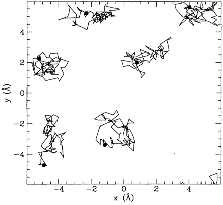
Hydrogen Molecule

$$ \begin{align} H &= -\frac{\nabla_1^2+\nabla_2^2}{2}+ \frac{1}{|\br_1-\br_2|}\\ &- \sum_{i=1,2}\left[\frac{1}{|\br_i-\hat{\mathbf{z}} R/2|} + \frac{1}{|\br_i+\hat{\mathbf{z}}R/2|}\right] \end{align} $$

• Spatial wavefunction again symmetric

• Equilibrium proton separation $R=1.401$, $E_0= -1.174476$

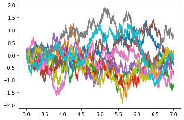
Exchange Processes

• At $R=8.5$ tunnelling events are visible

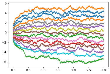
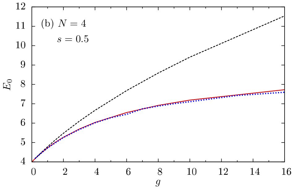
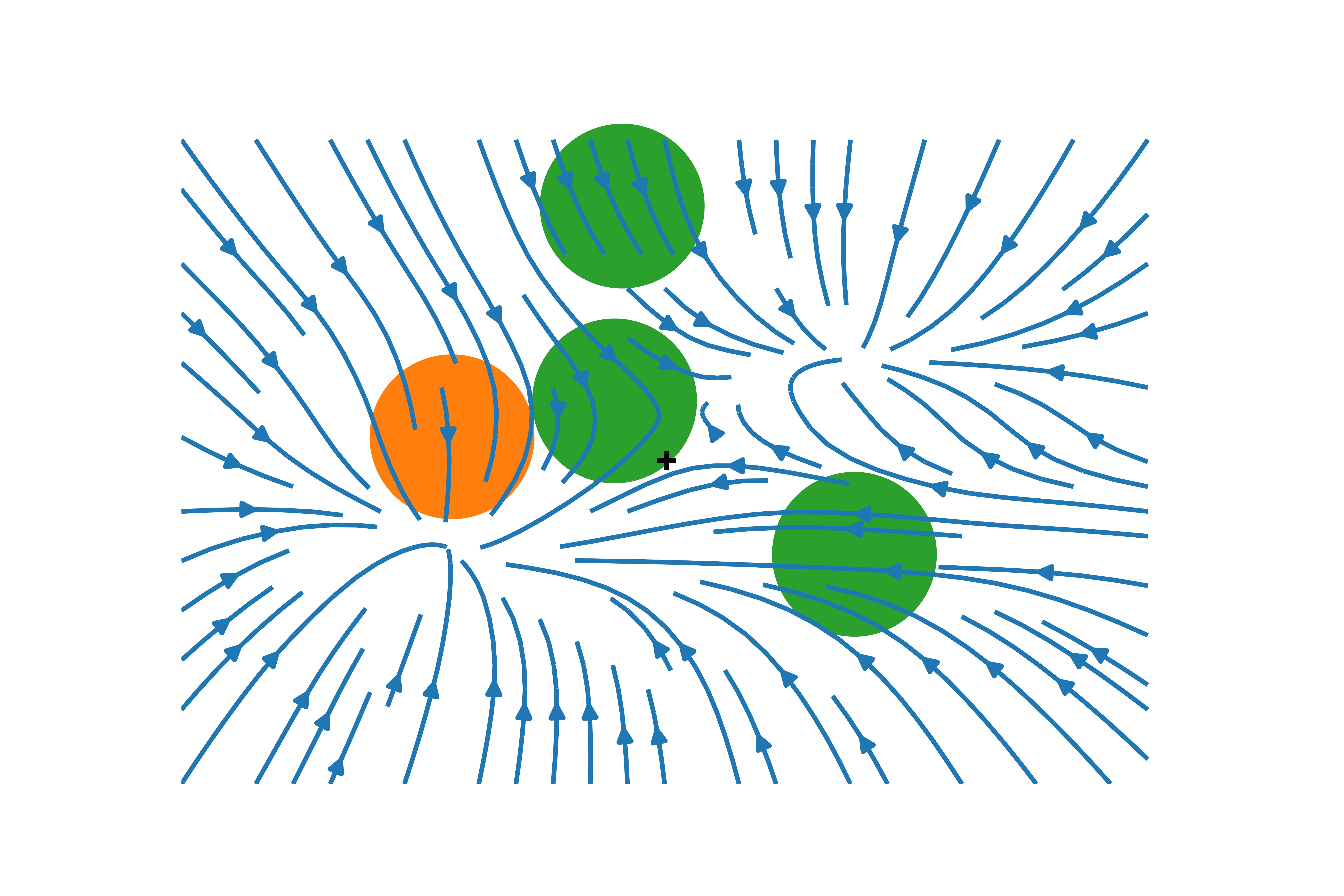
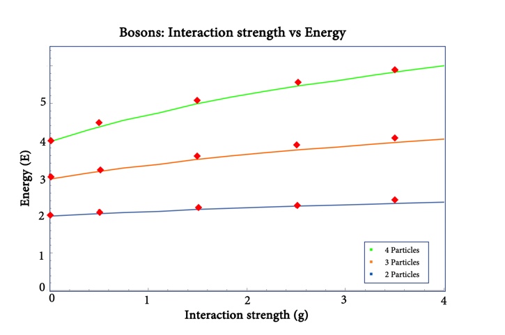
2D Gaussian Bosons

$$ \begin{align} H&=\frac{1}{2}\sum_i \left[\nabla_i^2 +\br_i^2\right]+\sum_{i<j}U(\br_i-\br_j)\\ U(\br) &=\frac{g}{\pi s^2}e^{-\br^2/s^2} \end{align} $$

• Mujal et al., PRA 2017 model for ultracold atoms

• Drift Visualization ($g=10$, $s=1/2$)

Outlook

• Excited states; angular momentum ↔ non-reversible drift

• Fermions?

• Lattice models

Next Up: Lattice Models

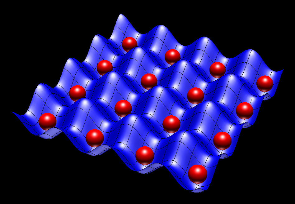
XY model

• On chain / square / cubic lattice

$$ \begin{align} \partial_t \Psi_{\Huge\circ\Huge\bullet\Huge\circ} &= \Psi_{\Huge\bullet\Huge\circ\Huge\circ}+\Psi_{\Huge\circ\Huge\circ\Huge\bullet}\\ &=\overbrace{ \Psi_{\Huge\bullet\Huge\circ\Huge\circ}+\Psi_{\Huge\circ\Huge\circ\Huge\bullet}-2\Psi_{\Huge\circ\Huge\bullet\Huge\circ}}^{\text{master / forward eq.}} +2 \Psi_{\Huge\circ\Huge\bullet\Huge\circ} \end{align} $$

• c.f. imaginary time Schrödinger

$$ \frac{\partial\psi(\br,t)}{\partial t} = \left[\frac{\nabla^2}{2}-V(\br_i)\right]\psi(\br,t) $$

• $\exists$ Feynamn–Kac representation!

Linearly Solvable MDPs

• Todorov (2017) introduced cost

$$ \ell(j,v) = q(j) + D_{\text{KL}}\left(v(\cdot|j) \middle\|\middle\| p(\cdot|j)\right) $$

• $v(j|k)$ is controlled dynamics, $p(j|k)$ is “passive dynamics”

• Bellman equation for the cost to go $\nu(j,t)$

$$ \nu(k,t) = \min_v\left[\ell(k,u) + \E_{j\sim u(\cdot|k)}\nu(j,t+1)\right] $$

• Transform to linear equation for desirability $\Psi(j,t) = \exp(-\nu(j,t))$

• Optimal dynamics

$$ u^*(j|k)=\frac{p(j|k)\Psi(j)}{\sum_{l}p(l|k)\Psi(l)}, $$

• Linear equation

$$ \Psi(k,t) = e^{-q(k)}\sum_{j}p(j|k)\Psi(j,t+1). $$

• Discrete imaginary time Schrödinger equation

Any model with FK formula has control rep.!