Space-time dual quantum circuits
Austen Lamacraft (Cambridge) and Pieter Claeys (Dresden)
austen.uk/#talks for slides
Motivation: kicked Ising model
- Time dependent Hamiltonian with kicks at $t=0,1,2,\ldots$
$$ \begin{aligned} H_{\text{KIM}}(t) = H_\text{I}[\mathbf{h}] + \sum_{m}\delta(t-n)H_\text{K}\\ H_\text{I}[\mathbf{h}]=\sum_{j=1}^L\left[J Z_j Z_{j+1} + h_j Z_j\right],\qquad H_\text{K} &= b\sum_{j=1}^L X_j \end{aligned} $$
- “Stroboscopic” form of $U(t)=\mathcal{T}\exp\left[-i\int^t H_{\text{KIM}}(t’) dt’\right]$
$$ \begin{aligned} U(n_+) &= \left[U(1_+)\right]^n,\qquad U(1_-) = K I_\mathbf{h}\\ I_\mathbf{h} &= e^{-iH_\text{I}[\mathbf{h}]}, \qquad K = e^{-iH_\text{K}} \end{aligned} $$
Unitary circuit
- Another class of discrete time dynamics
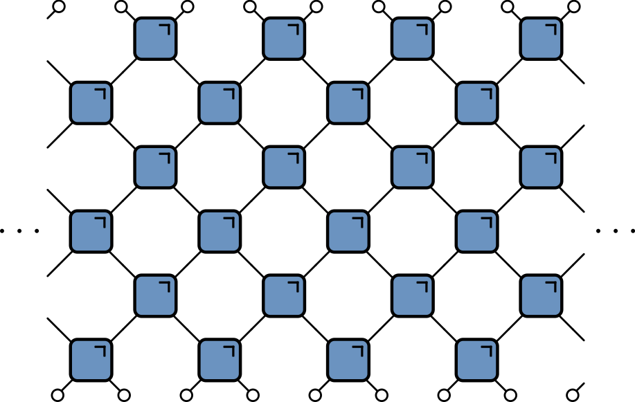
KIM as a circuit
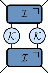
$$ \begin{aligned} \mathcal{K} &= \exp\left[-i b X\right]\\ \mathcal{I} &= \exp\left[-iJ Z_1 Z_2 -i \left(h_1 Z_1 + h_2 Z_2\right)/2\right] \end{aligned} $$
Expectation values
- Evaluate $\bra{\Psi}\mathcal{O}\ket{\Psi}=\bra{\Psi_0}\mathcal{U}^\dagger\mathcal{O}\mathcal{U}\ket{\Psi_0}$ for local $\mathcal{O}$
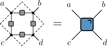
Folded picture
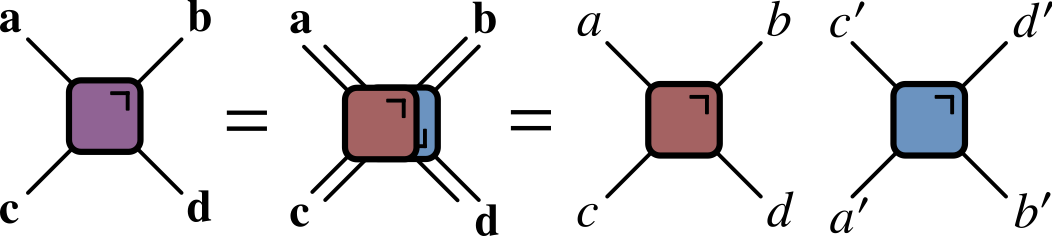
- After folding, lines correspond to two indices / 4 dimensions
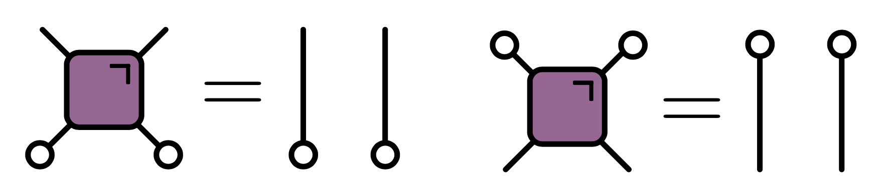
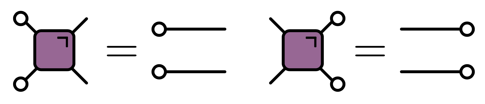
Unitarity in folded picture
- Circle denotes $\delta_{ab}$
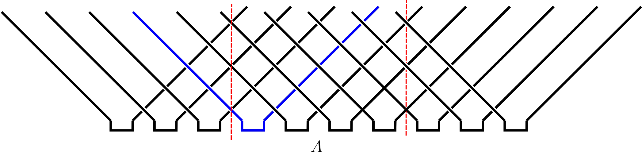
$\bra{\Psi}\mathcal{O}\ket{\Psi}$ in folded picture
- Emergence of “light cone”
Reduced density matrix
- Expectation values in region $A$ evaluated using reduced density matrix
$$ \rho_A = \operatorname{tr}_{\bar A}\left[\ket{\Psi}\bra{\Psi}\right]=\operatorname{tr}_{\bar A}\left[\mathcal{U}\ket{\Psi_0}\bra{\Psi_0}\mathcal{U}^\dagger\right] $$
Toy model: SWAP circuit
For a Bell pair consisting of qubits at sites $m$ and $n$:
If $n\in A$, $m\in\bar A$, $\rho_A$ has factor $\mathbb{1}_n$.
If $m, n\in A$ they contribute a factor $\ket{\Phi^+}_{nm}\bra{\Phi^+}_{nm}$ (pure)
Only first case contributes to
$ S_A = \min(4\lfloor t/2\rfloor, |A|) $bits
Dual unitary gates
- Impose additional restriction
$\rho_A$ via dual unitarity
- 8 sites; 4 layers; Bell pair initial state
- $\rho_A$ is unitary transformation of
$$ \mathbb{1}\otimes\mathbb{1}\otimes\mathbb{1}\otimes\mathbb{1}\otimes\mathbb{1}\otimes\mathbb{1}\otimes\mathbb{1}\otimes\mathbb{1} $$
Shallower…
- $\rho_A$ is unitary transformation of
$$ \mathbb{1}\otimes\mathbb{1}\ket{\Phi^+}\bra{\Phi^+}\otimes\ket{\Phi^+}\bra{\Phi^+}\otimes\mathbb{1}\otimes\mathbb{1} $$
General case
- RDM is unitary transformation of
$$ \rho_0=\overbrace{\frac{\mathbb{1}}{2}\otimes \frac{\mathbb{1}}{2} \cdots }^{t-1} \otimes\overbrace{\ket{\Phi^+}\bra{\Phi^+} \cdots }^{N_A/2-t+1 } \otimes \overbrace{\frac{\mathbb{1}}{2}\otimes \frac{\mathbb{1}}{2} \cdots }^{t-1} $$
RDM has $2^{\min(2t-2,N_A)}$ non-zero eigenvalues all equal to $\left(\frac{1}{2}\right)^{\min(2t-2,N_A)}$
Converse – maximal entanglement growth implies dual unitary gates – recently proved by Zhou and Harrow (2022)
Thermalization
After $N_A/2 + 1$ steps, reduced density matrix is $\propto \mathbb{1}$
All expectations (with $A$) take on infinite temperature value
The dual unitary family
$4\times 4$ unitaries are 16-dimensional
Family of dual unitaries is 14-dimensional
Includes kicked Ising model at particular values of couplings
Dual unitaries not “integrable” (except at special points) but have enough structure to allow many calculations
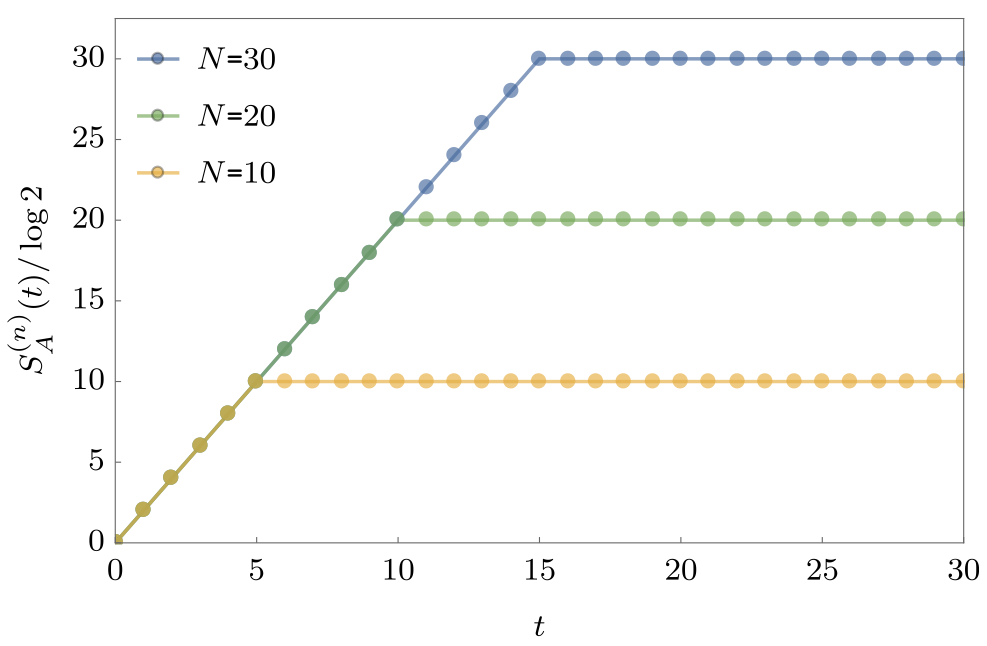
Entanglement Growth for Self-Dual KIM
- Bertini, Kos, Prosen (2019) found that when $|J|=|b|=\pi/4$
$$ \lim_{L\to\infty} S_A =\min(2t-2,N_A)\log 2, $$
- Any $h_j$; initial $Z_j$ product state
‘KIM’ property
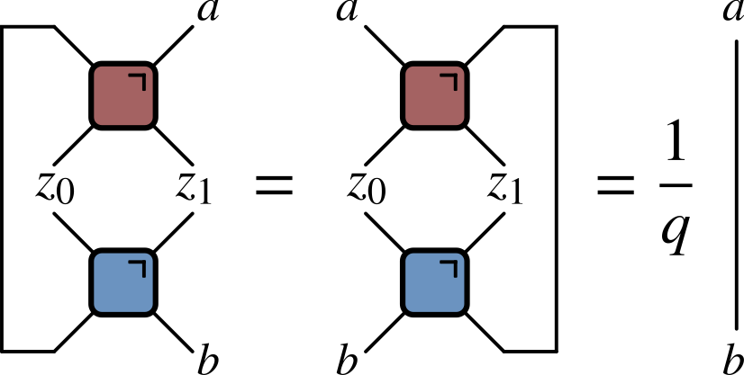
($q=2$ here) Not satisfied by e.g. $\operatorname{SWAP}$
Maps product states to maximally entangled (Bell) states
Product initial states also work for KIM!
Piroli et al (2020) studied more general initial states
Correlation functions
- Infinite temperature correlator $\tr\left[\sigma^\alpha_x(x,t)\sigma^\beta(y,0)\right]$
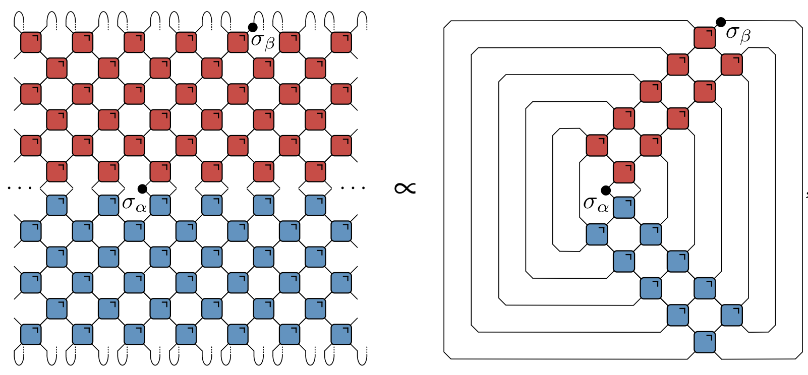
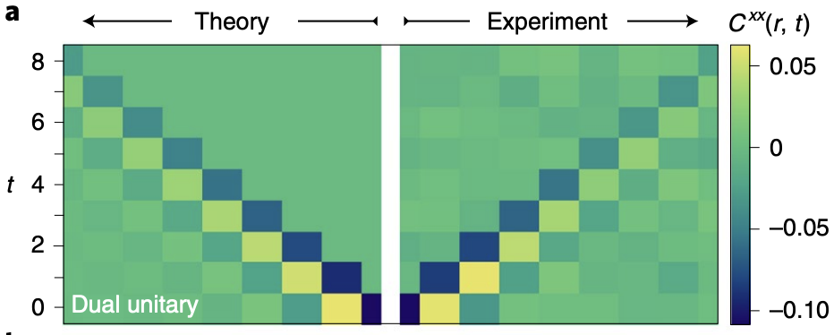
- Bertini, Kos, and Prosen (2019): dual unitarity means correlations vanish inside light cone!
Quantinuum experiment
- Correlations measured in SDKIM by Chertkov et al. (2022)
Outline
New directions:
Space-time dual models from ZX calculus and Hadamards
Cat maps, Clifford gates and the classical limit
Curiosity:
- Discrete Lorentz invariance
ZX Calculus
- Calculus of “special” tensors
- See also van der Wetering (2020)
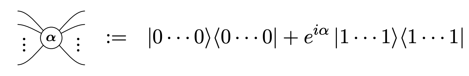
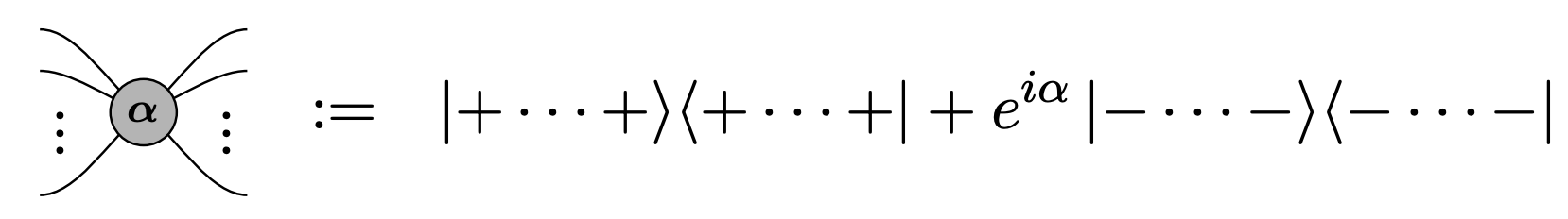
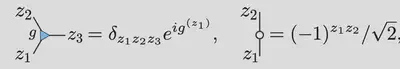
Basic ingredients: Z and X tensors (“spiders”)
$$ |0\rangle=\left(\begin{array}{l} 1 \\ 0 \end{array}\right) \quad|1\rangle=\left(\begin{array}{l} 0 \\ 1 \end{array}\right) \quad|+\rangle=\frac{1}{\sqrt{2}}\left(\begin{array}{l} 1 \\ 1 \end{array}\right) \quad|-\rangle=\frac{1}{\sqrt{2}}\left(\begin{array}{c} 1 \\ -1 \end{array}\right) $$
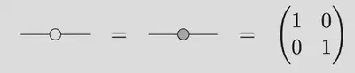
Simplest examples
- Identity
- CNOT

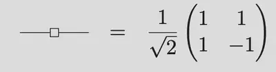
Colour changing with Hadamards
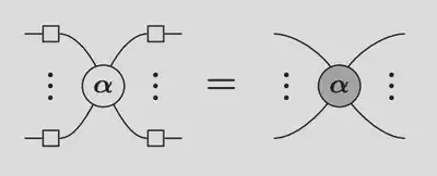
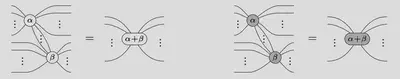
Spider fusion
Follows that $n$-leg spider is isometry: $\mathbb{C}^2\longrightarrow \mathbb{C}^{2^{n-1}}$
Contract $n-1$ legs of $\alpha$ and $\beta=-\alpha$
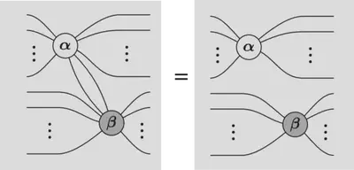
Hopf rule aka “leg chopping”
Example: Liu and Ho (2023)
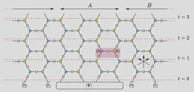
Rewrite in ZX language

- CNOTs (East model, Bertini et al. (2023)) + phases on each spider
Unitarity of Liu–Ho gate

- Spider fusion: 🟢—🟢 = 🟢 and 🔴—🔴 = 🔴 then leg chopping
- Not dual unitary but overall circuit triunitary (Jonay et al. (2021))

### Three light rays / null directions
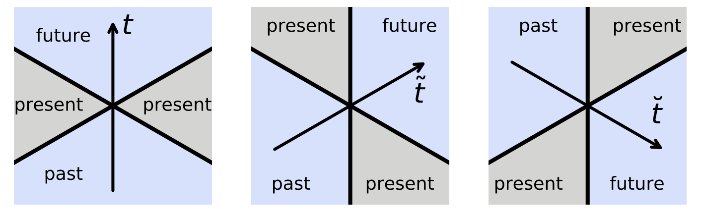
- Correlations nonzero in three directions!
- Apply to 🟢 🔴 🟢 🔴 🟢 🔴 initial state

- Spider fusion

- Isometries along bottom are origin of solvability
- See Liu and Ho (2023) for much more!
Circuits based on Hadamard gates
- Recall KIM has circuit representation
$$ \begin{aligned} \mathcal{K} &= \exp\left[-i b X\right]\\ \mathcal{I} &= \exp\left[-iJ Z_1 Z_2 -i \left(h_1 Z_1 + h_2 Z_2\right)/2\right] \end{aligned} $$
- At $|J|=|b|=\pi/4$ model is dual unitary
“Seeing” dual unitarity
- At the dual unitary point $b=\pm i\pi/4$
$$ \mathcal{K} = \exp\left[\pm i \frac{\pi}{4} X\right]=\frac{1}{\sqrt{2}}\begin{pmatrix} 1 & \pm i \\ \pm i & 1 \end{pmatrix} $$
Is $\propto$ Hadamard matrix: $|H_{ij}|=1$ with $H^\dagger H = d\mathbb{1}$
Can be interpreted as diagonal phases when “viewed sideways”

- Back to lattice spin model picture
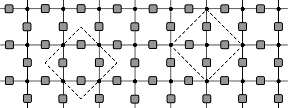

$$ U = \mathcal{N}\sum_{z_i\in \mathbb{Z}_d}\prod_{<i,j>} u_{ij}(z_i, z_j) $$
$u_{ij}(z_i, z_j): \mathbb{Z}_d\times \mathbb{Z}_d\longrightarrow U(1)$
$z_i=\omega_d^{n_i}$ for $n_i=0,\ldots d-1$, with $\omega_d = \exp(2\pi i/d)$
$$ U = \mathcal{N}\sum_{z_i\in \mathbb{Z}_d}\prod_{<i,j>} u_{ij}(z_i, z_j) $$
When does this describe unitary evolution (vertically)?
Single row $U_{\text{row }t}$ corresponds to diagonal operator

$$ \braket{z_{1:N,t}|U_{\text{row }t}|z_{1:N,t}} = \prod_{x=1}^N u_\text{H}(z_{x,t},z_{x+1,t}) $$
- Unitary since $u_\text{H}$ are phases

- Vertical bonds correspond to operators $u_\text{V}$ with matrix elements
$$ u_\text{V}(z_i,z_j)=\braket{z_i|u_\text{V}|z_j} $$
- Also unitary up to a multiplicative factor i.e. $u_\text{V}$ is Hadamard!
In the same way, space-like evolution is unitary if $u_\text{H}$ is Hadamard
If both $u_\text{V}$ and $u_\text{H}$ are Hadamard (e.g. SKDI): unitary evolution in both space and time or space-time duality (Gutkin et al. (2020))
Hadamard matrices
- Simple and important example is Fourier matrix (performs DFT)
$$ \left(F_d\right)_{jk} = \exp\left(2\pi ijk/d\right)\qquad j,k=0,\ldots, d-1 $$
$H$ and
$H'$are equivalent if$$ H' = D_1P_1 H P_2 D_2 $$$D_{1,2}$ are diagonal unitaries and $P_{1,2}$ permutations
If $D_1=D_2=\mathbb{1}$ $H$ and
$H'$are permutation equivalent
Dephased form of a Hadamard matrix has first row and column all 1
Two Hadamard matrices with same dephased form are equivalent
$$ \begin{align*} H_\text{deph} &= D_1 H D_2\\ D_1&= \operatorname{diag}(\bar H_{11},\bar H_{21},\ldots \bar H_{d1})\\ D_2&= \operatorname{diag}(1,H_{11}\bar H_{12},\ldots H_{11}\bar H_{1d}) \end{align*} $$
$d=2,3$ and $5$: all complex Hadamard matrices equivalent to $F_d$
$$ F_2 = \begin{pmatrix} 1 & 1 \\ 1 & -1 \end{pmatrix} $$Equivalent to self-dual Ising kick matrix
$$ K_{2} =\begin{pmatrix} 1 & i \\ i & 1 \end{pmatrix}= \begin{pmatrix} 1 & 0\\ 0 & i \end{pmatrix} F_2\begin{pmatrix} 1 & 0\\ 0 & i \end{pmatrix} $$
- As a phase function
$$ K_{2}(z_i, z_j) = e^{i\pi/4}\exp\left(-\frac{i\pi}{4} z_i z_j\right) $$ $$ F_{2}(z_i, z_j) = e^{i\pi/4}\exp\left(\frac{i\pi}{4} \left[z_i z_j-z_i-z_j\right]\right) $$
- For $d=3$
$$ F_3 = \begin{pmatrix} 1 & 1 & 1 \\ 1 & \omega_3 & \omega_3^2 \\ 1 & \omega_3^2 & \omega_3 \end{pmatrix} $$
- Equivalent to
$$ K_3 = \begin{pmatrix} 1 & \omega_3 & \omega_3 \\ \omega_3 & 1 & \omega_3 \\ \omega_3 & \omega_3 & 1 \\ \end{pmatrix} $$
- Tensor product of Hadamards is Hadamard e.g.
$$ F_2\otimes F_2 = \begin{pmatrix} 1 & 1 & 1 & 1 \\ 1 & -1 & 1 & -1 \\ 1 & 1 & -1 & -1 \\ 1 & -1 & -1 & 1 \end{pmatrix} $$
- Permutation inequivalent to $F_4$. Full orbit of inequivalent Hadamards
$$ F_4^{(1)}(a)=\left[\begin{array}{cccc} 1 & 1 & 1 & 1 \\ 1 & i e^{i a} & -1 & -i e^{i a} \\ 1 & -1 & 1 & -1 \\ 1 & -i e^{i a} & -1 & i e^{i a} \end{array}\right]\qquad a \in [0,\pi) $$
- $F_4^{(1)}(0)=F_4$ and $F_4^{(1)}(\pm\pi/4)$ is perm equivalent to $F_2\otimes F_2$
Cat maps, Clifford gates and the classical limit
Generalized Pauli matrices
$$ \begin{align*} Z_d = \begin{pmatrix} 1 & 0 & 0 & \cdots & 0\\ 0 & \omega_d & 0 & \cdots & 0\\ \cdots & \cdots & \cdots & \cdots & \cdots \\ 0 & 0 & 0 & \cdots & \omega_d^{d-1} \end{pmatrix}\\ X_d = \begin{pmatrix} 0 & 1 & 0 & \cdots & 0\\ 0 & 0 & 1 & \cdots & 0\\ \cdots & \cdots & \cdots & \cdots & \cdots \\ 1 & 0 & 0 & \cdots & 0 \end{pmatrix} \end{align*} $$
Satsify $Z_d^d=X_d^d=\mathbb{1}$ and Weyl relation $X_d Z_d = \omega_d Z_d X_d$
$Z^a X^b$ with $a,b=0,\ldots d-1$ form basis for local operators
Quantum mechanical analogue of phase space torus $$ Z= e^{2\pi i q}\qquad X=e^{2\pi ip} $$
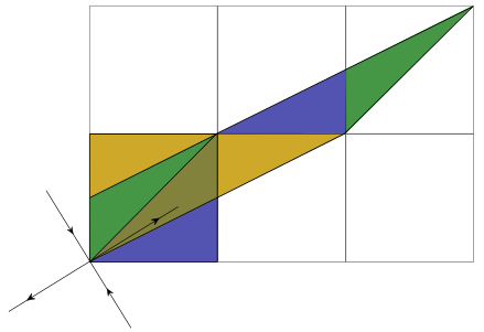
Conjugating by Fourier matrix $$ F Z^a X^b F^\dagger = X^{a}Z^{-b} $$ like $-\pi/2$ rotation of torus: $(q,p)\longrightarrow (p,-q)$
Cat maps
$$ C_{jk}(\alpha,\delta)\equiv \exp\left(\frac{2\pi i}{d}\left[\frac{\alpha j^2}{2} + jk + \frac{\delta k^2}{2}\right]\right)\qquad \alpha,\delta\in \mathbb{Z} $$
Area preserving (symplectic) linear map on torus
$$ \begin{align*} \begin{pmatrix} q \\ p \end{pmatrix}&\longrightarrow \begin{pmatrix} q' \\ p' \end{pmatrix} = T \begin{pmatrix} q \\ p \end{pmatrix}\qquad \mod 1\nonumber\\ T &= \begin{pmatrix} \alpha & \beta \\ \gamma & \delta \end{pmatrix}\qquad \alpha,\beta,\gamma,\delta\in\mathbb{Z},\qquad \alpha\delta-\beta\gamma=1 \end{align*} $$$C_{jk}(\alpha,\delta)$ has $\beta=1$ and is Clifford:
$Z^a X^b\longrightarrow Z^{a'} X^{b'}$Quantum cat maps first studied by Hannay and Berry (1980) as quantum analogs of classical Arnold cat maps
Arnold’s cat map
$$ T:\begin{pmatrix} q \\ p \end{pmatrix}\longrightarrow \begin{pmatrix} \alpha & 1 \\ \alpha\delta - 1 & \delta \end{pmatrix} \begin{pmatrix} q \\ p \end{pmatrix}\qquad \mod 1 $$
- Chaotic when one Lyapunov exponent exceeds one for $|\alpha+\delta|>2$.
$$ \begin{align*} T &= \begin{pmatrix} 2 & 1 \\ 3 & 2 \end{pmatrix}: C_{jk}(2,2) = \exp\left(\frac{2\pi i}{d}\left[j^2+k^2+jk\right]\right)\text{ (hyperbolic)}\nonumber\\ T &= \begin{pmatrix} -1 & 1 \\ 0 & -1 \end{pmatrix}: C_{jk}(-1,-1) = \exp\left(-\frac{i\pi}{d}\left[j-k\right]^2\right) \text{ (parabolic)} \end{align*} $$
- Find update of general Pauli
$$ \prod_{x=1}^N Z^{a_{x,t}}X^{b_{x,t}}\qquad a_{x,t}, b_{x,t}\in \mathbb{Z}_d. $$
- Taking $u_\text{H}=F$ and $u_\text{V}=C(\alpha,\delta)$ (H then V)
$$ \begin{align*} a_{x,t+1} &= \alpha(a_{x,t}-b_{x-1,t}-b_{x+1,t}) + (\alpha\delta -1)b_{x,t}\nonumber\\ b_{x,t+1} &= a_{x,t} - b_{x-1,t} - b_{x+1,t}+\delta b_{x,t} \end{align*}\mod d $$
- “Hamiltonian” form of equations of motion
- Second difference “Lagrangian” formulation
$$ \begin{align*} \left[\Delta b\right]_{x,t} &= (\alpha + \delta - 4)b_{x,t}\qquad \mod d\nonumber\\ \left[\Delta b\right]_{x,t} &\equiv b_{x,t+1} + b_{x+1,t-1} + b_{x+1,t} + b_{x-1,t} - 4b_{x,t} \end{align*} $$
Symmetry between space and time is evident
Taking $u_\text{H}=F^\dagger$ and $u_\text{V}=C(\alpha,\delta)$
$$ \begin{align*} \left[\square b\right]_{x,t} &= (\alpha + \delta)b_{x,t}\qquad \mod d\nonumber\\ \left[\square b\right]_{x,t} &\equiv b_{x,t+1} + b_{x+1,t-1} - b_{x+1,t} - b_{x-1,t} \end{align*} $$
- For $\alpha=\delta=0$ particularly simple form
$$ \begin{align*} \left[\square b\right]_{x,t} &= 0 \end{align*} $$
- Left and right propagating solutions
$$ \begin{align*} a^R_{x,t} &= r_{x-t} \qquad b^R_{x,t} = -r_{x-t-1}\nonumber\\ a^L_{x,t} &= l_{x+t} \qquad b^L_{x,t} = -l_{x+t+1} \end{align*} $$
General case: (Gütschow et al. (2010))
Fourier transform of equation of motion
$$ M(u, u^{-1}) = \begin{pmatrix} \alpha & (\alpha\delta - 1) + \alpha(u + u^{-1}) \\ 1 & \delta + u + u^{-1} \end{pmatrix} $$
$\operatorname{tr}M = \alpha + \delta + u + u^{-1}$ determines behaviour
$\alpha+\delta=0$: glider automaton otherwise fractal
- Example: $d=3$, $u_\text{V}=C(1,0)$
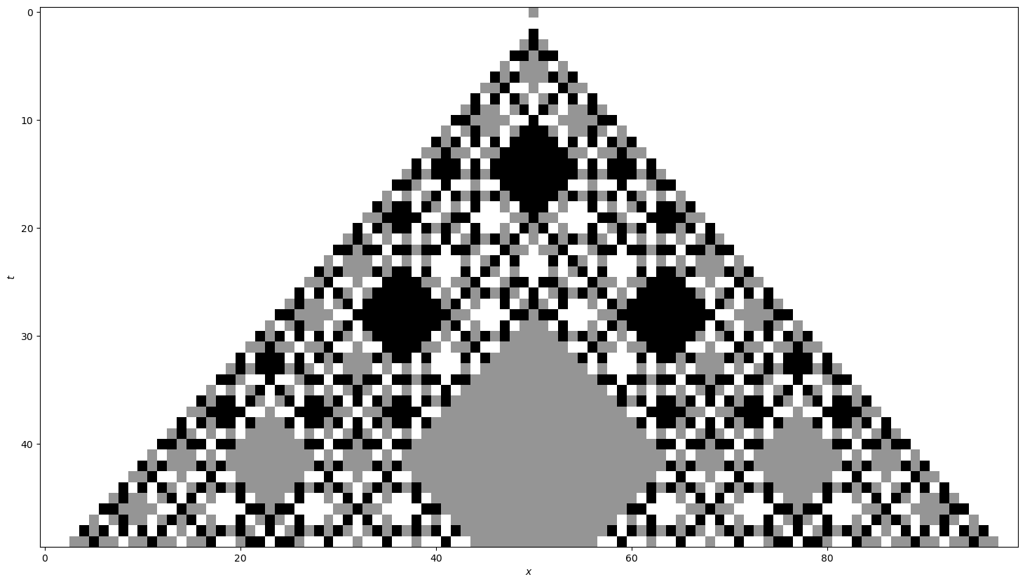
- Local correlations vanish quickly!
Spatiotemporal cat
Gutkin and Osipov (2016) define map on $N$ copies of torus
Coupling between sites via
$$ \begin{align*} x_{n}&\longrightarrow x_n \\ y_{n}&\longrightarrow y_n - x_{n-1} - x_{n+1} - V'(x_n) \end{align*}\qquad \mod 1 $$Generated by Hamiltonian (NB $V(x)$ periodic) $$ H_\text{c} = \sum_n \left[x_{n} x_{n+1} + V(x_n)\right] $$
Alternate with cat maps $\mathcal{K}_n$ on each site
Lagrangian picture
- “Momenta” $y_n$ can be eliminated to give two-step (Lagrangian) recurrence for $x_{n,t}$:
$$ [\Delta x]_{n,t} = (a+b-4)x_{n,t} - V'(x_{nt})-m_{n,t} \mod 1 $$winding numbers $m_{n,t}$ chosen to ensure $x_{n,t}$ stays in the unit interval and $\Delta$ is the 2D Laplacian
Correlations
Hu and Rosenhaus (2022), Fouxon and Gutkin (2022): explicit results for two and three site correlations.
Correlations vanish for $t>\ell$, support of observable
Christopoulos et al. (2023) and Lakshminarayan (2023) for correlations in other models
Lotkov et al. (2022)
Floquet dynamics for $d=3$
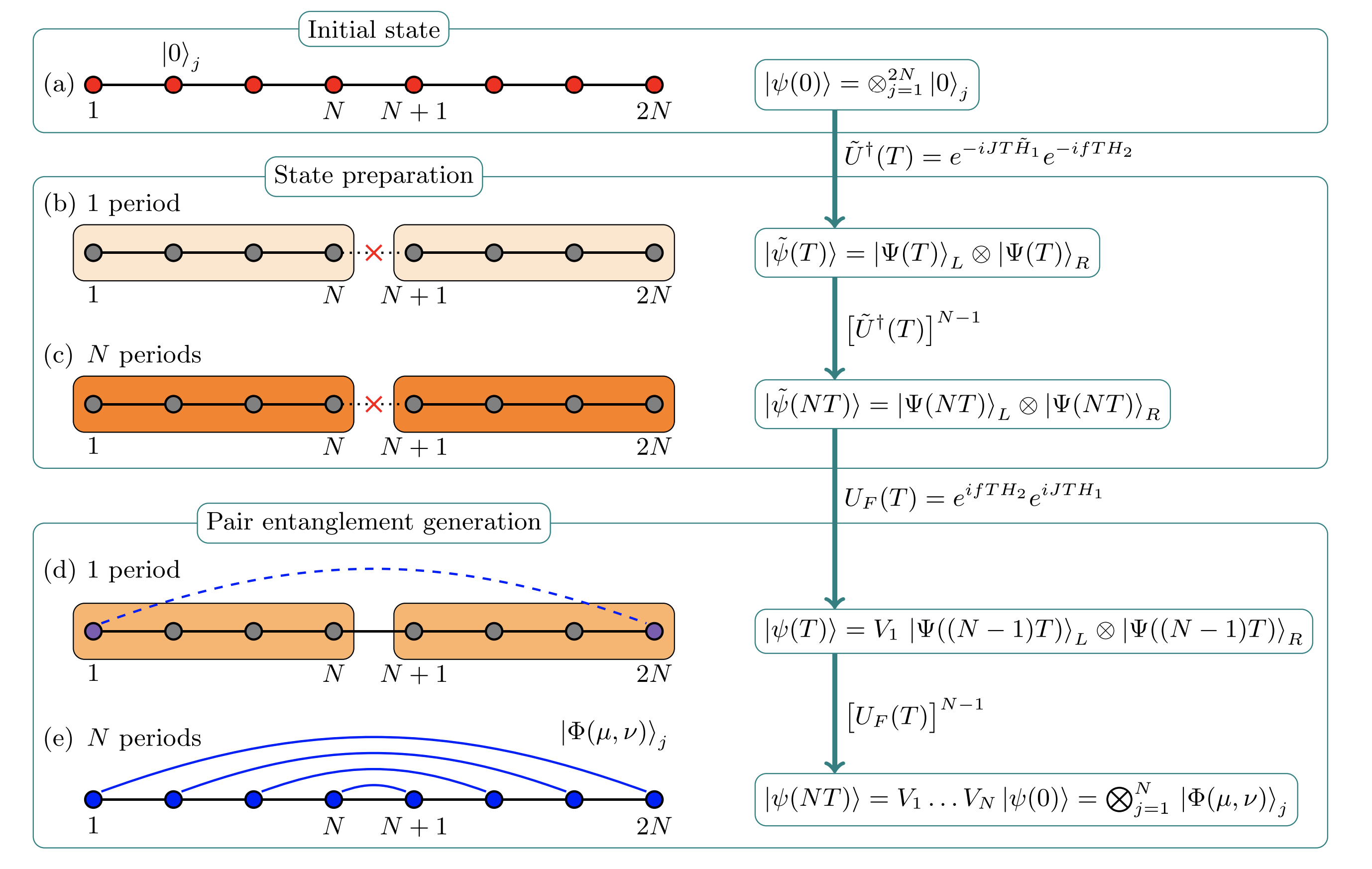
$$ \begin{align*} H_1 &= \sum_{j=1}^{2N-1}\left(X_j^{\dagger}X_{j+1}+X_j X^{\dagger}_{j+1}\right)\\ H_2 &= \sum_{j=1}^{2N}\left(Z_j+Z_j^{\dagger}\right)\\ U_F &= e^{ifTH_2}e^{iJTH_1} \end{align*} $$Integrability conjectured for $fT = JT = \alpha_m$, with $\alpha_m = \frac{2\pi}{9}(2\ell-m)$, with $m=\pm 1$ and $\ell \in \mathbb{Z}$.
Integrability subsequently established by Miao and Vernier (2023)
- Long range entanglement generation in integrable case
- Integrable case corresponds to
$$ \begin{align*} v_\text{H} = \begin{pmatrix} 1 & \omega & \omega \\ \omega & 1 & \omega \\ \omega & \omega & 1 \end{pmatrix} \qquad v_\text{V} = \begin{pmatrix} 1 & \omega^2 & \omega^2 \\ \omega^2 & 1 & \omega^2 \\ \omega^2 & \omega^2 & 1 \end{pmatrix}=\bar v_\text{H} \end{align*} $$
$v_\text{H}$ dephases to $F$, so this is equivalent to $v_\text{H}=F$, $v_\text{V}=F^\dagger$
Hence, ballistic propagation of operators
Diagrammatic derivation of rainbow state
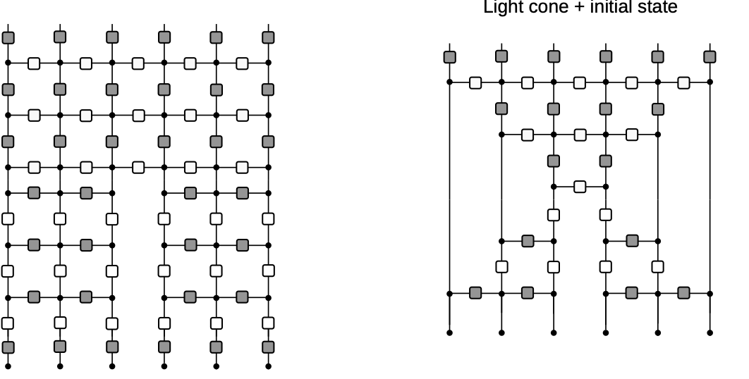
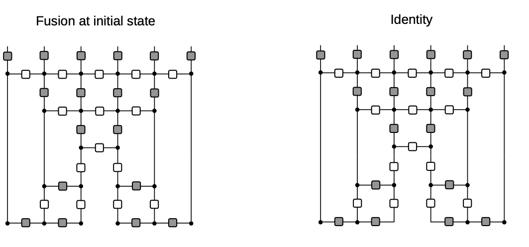
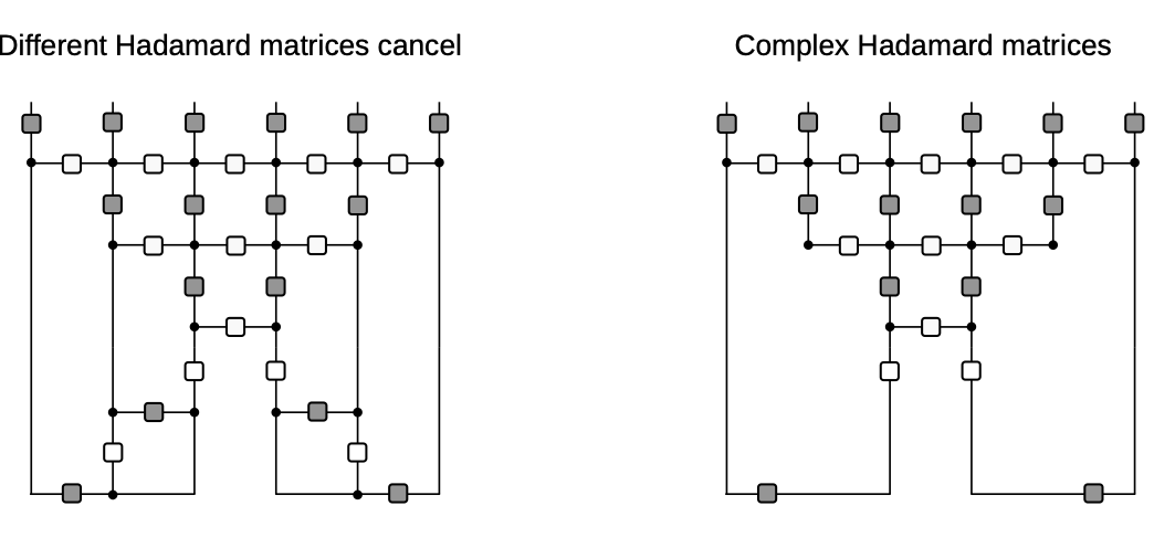
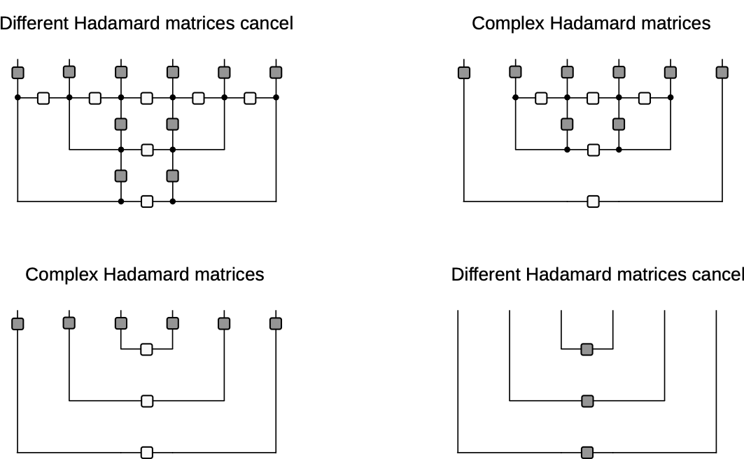
- Nonintegrable case
$$ v_\text{H} = v_\text{V} = \begin{pmatrix} 1 & \omega & \omega \\ \omega & 1 & \omega \\ \omega & \omega & 1 \end{pmatrix} $$
- Fractal operator dynamics
Three dimensions
Questions
Do integrable dual unitary circuits have “trivial” dynamics?
Is Fourier circuit model integrable in the usual sense (for $d>3$?)
Can we connect fractal behaviour of cats at finite $d$ to classical limit?
Last thing: Lorentz symmetry

$$ \color{red}\Lambda\color{green}\mathcal{T} \color{black}=\color{green} \mathcal{T}'\color{red}\Lambda $$
$$ \color{red}\Lambda\color{green}\mathcal{T}\color{red}\Lambda^\dagger \color{black}=\color{green} \mathcal{T}' $$
- Masanes suggests (arXiv:2301.02825) DU circuits connected to CFTs