$$ \nonumber \newcommand{\bra}[1]{\langle{#1}\rvert} \newcommand{\ket}[1]{\lvert{#1}\rangle} \newcommand{\braket}[2]{\langle{#1}\vert{#2}\rangle} \newcommand{\br}{\mathbf{r}} \newcommand{\bR}{\mathbf{R}} \newcommand{\bp}{\mathbf{p}} \newcommand{\bk}{\mathbf{k}} \newcommand{\bq}{\mathbf{q}} \newcommand{\bv}{\mathbf{v}} \newcommand{\bx}{\mathbf{x}} \newcommand{\bz}{\mathbf{z}} \DeclareMathOperator*{\E}{\mathbb{E}} $$
Absence of superdiffusion in certain random spin models
Work with Pieter Claeys and Jonah Herzog-Arbeitman

Embarrassingly simple question
What is nature of spin transport in Heisenberg chain? $$ H = \sum_j \left[X_j X_{j+1}+Y_j Y_{j+1}+ Z_j Z_{j+1}\right] $$
All 3 components conserved
(Naive) expectation: diffusion at $T>0$ (including $T=\infty$)
Simple?
- Except: nonabelian, low dimension, integrability, …
Recent predictions
(Very) good evidence for KPZ(ish) behavior $\ell\sim t^{2/3}$ in integrable, nonabelian models, classical and quantum
Recent review Bulchandani, Gopalakrishnan, Ilievski (2021)
- De Nardis et al. (2020) $D(t)\sim (\log t)^{4/3}$ in classical Heisenberg chain
- McRoberts et al. (2021) on classical FM (blue) and AFM (orange)
- At finite $T$ FM looks anomalous (KPZish); AFM looks normal
- De Nardis et al. (2021) $D(t)\sim \log t$ with noisy exchange coupling
Lack of theory tools
No integrability; “weak integrability breaking” in its infancy
Absence of small parameters: exchange coupling $J$ is only scale
This work: noisy exchange coupling
\begin{equation} H = \sum_{j,a} \left[(J + \xi_j(t))\sigma^a_j \sigma^a_{j+1}\right] \end{equation}
Studied numerically in De Nardis et al. (2021)
$SU(2)$ invariance but no energy conservation
Expect (nonabelian) hydrodynamics of spin modes to play major role
Can develop perturbation theory in $J$
Correlation function
Spin-1/2 chain of $N$ sites with spin $\boldsymbol{\sigma}_j=(X_j, Y_j, Z_j)$ at site $j$
Infinite temperature spin-spin correlator
$$ C^{ab}_{jk}(t)\equiv\frac{1}{2^N}\mathop{\mathrm{tr}}\left[\sigma^a_j(0) \sigma^b_k(t)\right]\qquad \sigma^b_k(t)=\mathcal{U}^\dagger_t \sigma^b_k \mathcal{U}_t. $$
$SU(2)$ invariance: $C^{ab}_{jk}(t)\equiv\delta_{ab}C_{jk}(t)$ with $\sum_{k=1}^N C_{jk}(t)=1$
From now on fix $a=b=z$
Expansion in Pauli basis
$$ Z_j(t)= \sum_{\mu_{1:N}={0,1,2,3}^N} \mathcal{C}{\mu{1:N}}(t) \sigma_1^{\mu_1}\otimes\cdots \sigma_N^{\mu_N},\qquad \sigma^\mu = (\mathbb{1},X,Y,Z) $$
- With initial condition
$$ \begin{equation} \mathcal{C}_{\mu_{1:N}}(0)=\begin{cases} 1 & \mu_j=z, \mu_k=0,\forall k\neq j \\ 0 & \text{otherwise}, \end{cases} \end{equation} $$
- Spin correlation function is $C_{jk}(t) = \mathcal{C}_{0\cdots \mu_k=z \cdots 0}(t)$

Model
- Fluctuating exchange coupling gives stochastic Schrödinger equation
\begin{equation}\label{eq:sse} d\ket{\psi} = \sum_j \left[-i(J dt + \sqrt{\eta}dW_j)P_{j,j+1}-\frac{\eta}{2}dt\right]\ket{\psi}. \end{equation}
$P_{j,j+1}=\frac{1}{2}\left[1+\sum_a \sigma^a_j \sigma^a_{j+1}\right]$ is exchange operator
$W_j$ independent Brownian motions (white noise $\propto dW_j$)
Itô stochastic differential equation: last term preserves $\braket{\psi}{\psi}$
Operator dynamics
- Heisenberg equation of motion ($\eta=1$)
\begin{multline}\label{eq:hberg} d\mathcal{O} = \sum_j \left[i\left(J dt + dW_j\right)\left[P_{j,j+1},\mathcal{O}\right]+dt\left(P_{j,j+1}\mathcal{O}P_{j,j+1}-\mathcal{O}\right)\right]. \end{multline}
- $\bar{\mathcal{O}}\equiv\E \mathcal{O}$ obeys the (adjoint) Lindblad equation
\begin{equation} \frac{d\bar{\mathcal{O}}}{dt} = \sum_j \left[iJ \left[P_{j,j+1},\bar{\mathcal{O}}\right]+\left(P_{j,j+1}\bar{\mathcal{O}}P_{j,j+1}-\bar{\mathcal{O}}\right)\right]. \label{eq:eom} \end{equation}
Circuit viewpoint
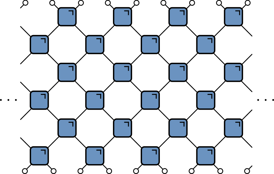
- $SU(2)$ preserving gate
$$ U_{j,j+1} = \cos\theta \mathbb{1}{j,j+1} - i\sin\theta P{j.j+1} $$
Operator Dynamics
$$ U_{j,j+1} = \cos\theta \mathbb{1}{j,j+1} - i\sin\theta P{j.j+1} $$
\begin{multline} \mathcal{O} \longrightarrow U^\dagger_{j,j+1}\mathcal{O}U_{j,j+1} = \cos^2\theta \, \mathcal{O} + \sin^2\theta \, P_{j.j+1}\mathcal{O} P_{j.j+1} \\ +i\sin\theta\cos\theta \left[P_{j.j+1}, \mathcal{O}\right] \end{multline}
- Take distribution $\theta=\pm \theta_0$ with $p(\theta_0)-p(-\theta_0)\equiv \delta > 0$
Average dynamics
\begin{multline} \overline{U^\dagger_{j,j+1}\mathcal{O}U_{j,j+1}} = \cos^2\theta_0 \, \mathcal{O} + \sin^2\theta_0 \, P_{j.j+1}\mathcal{O} P_{j.j+1} \\ +i\delta \sin\theta_0\cos\theta_0 \left[P_{j.j+1}, \mathcal{O}\right] \end{multline}
Interpretation:
- Operators on sites $j$ and $j+1$ switch with probability $\sin^2\theta_0$
- Asymmetry $\delta$ governs strength of “quantum” dynamics
Taking $\theta_0=\sqrt{dt}$, $\delta= J\sqrt{dt}$ gives continuous time evolution
Back to continuous time
$$ \frac{d\bar{\mathcal{O}}}{dt} = \sum_j \left[iJ \left[P_{j,j+1},\bar{\mathcal{O}}\right]+\left(P_{j,j+1}\bar{\mathcal{O}}P_{j,j+1}-\bar{\mathcal{O}}\right)\right]. $$
$J=0$: master equation describing random adjacent transpositions
Preserves subspaces corresponding to fixed numbers of each of the $\sigma^\mu$: 1 operator sector, 2 operator sector, …
$J=0$: 1 operator sector
- Writing $\mathcal{C}^a_{0\cdots \mu_k=a\cdots 0}\equiv C^a_k$ we have equation of motion
$$ \partial_t C^a_k = C^a_{k+1} + C^a_{k-1} - 2 C^a_k\equiv \Delta_k C^a_k $$
- Diffusion of single $\sigma^a$ ($\Delta_k$ is 1D discrete Laplacian)

$J=0$: 2 operator sector
- $C^{bc}_{j,k}\equiv \mathcal{C}_{0\cdots \mu_j=b\cdots \mu_k=c\cdots 0}$
$$ \partial_t C^{xy}_{m,n}= \Delta_m C^{xy}_{m,n}+ \Delta_n C^{xy}_{m,n} + \delta_{|m-n|-1}C^{xy}_{m,n} $$
- Last term plus condition $C^{xy}_{m,m}=0$ from hardcore condition

Perturbation theory
$$ \frac{d\bar{\mathcal{O}}}{dt} = \sum_j \left[iJ \left[P_{j,j+1},\bar{\mathcal{O}}\right]+\left(P_{j,j+1}\bar{\mathcal{O}}P_{j,j+1}-\bar{\mathcal{O}}\right)\right]. $$
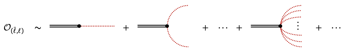
\begin{align} i[P,\sigma^a\otimes 1]&=-\epsilon^{abc}\sigma^b\otimes\sigma^c\nonumber\\ i[P,1\otimes \sigma^a]&=\epsilon^{abc}\sigma^b\otimes\sigma^c\nonumber\\ i[P,\sigma^a\otimes \sigma^b]&=\epsilon^{abc}\left(\sigma^c\otimes 1- 1\otimes \sigma^c\right). \label{eq:split-merge} \end{align}
Sum of first two expressions vanishes by spin conservation
Describe operator “splitting” ($1\to 2$) and “merging” ($2\to 1$).
Equation of motion
- In component form
$$ \begin{align} \partial_t \mathcal{C}_{\mu_{1:N}} = \sum_j \left[J\epsilon_{\alpha\beta \mu_j \mu_{j+1}} \mathcal{C}_{\mu_1\cdots \alpha\beta \cdots \mu_N} + \mathcal{C}_{\mu_1\cdots \mu_{j+1}\mu_j \cdots \mu_N} - \mathcal{C}_{\mu_1\cdots \mu_{j}\mu_{j+1} \cdots \mu_N}\right]. \end{align} $$
Simple approximation
- 1 and 2 operator sectors, dropping coupling to higher sectors
$$ \begin{align} \partial_t C^z_n = J\left[C^{xy}_{n-1,n}-C^{xy}_{n,n-1}-C^{xy}_{n,n+1}+C^{xy}_{n+1,n}\right] +\Delta_n C^z_n, \end{align} $$
$$ \begin{align} \partial_t C^{xy}_{m,n}& = J \left[\delta_{m+1,n}\left(C^z_m-C^z_{m+1}\right)+\delta_{m,n+1}\left(C^z_{n+1}-C^z_n\right)\right] \nonumber\\ &\qquad+\Delta_m C^{xy}_{m,n}+ \Delta_n C^{xy}_{m,n} + \delta_{|m-n|-1}C^{xy}_{m,n} \end{align} $$

Result for correlator
- $C^z(\eta,\omega)=\left[i\omega - \Omega(\eta)-\Sigma(\eta,\omega)\right]^{-1}$ in terms of self-energy

\begin{equation} \Sigma(\eta,\omega) = \frac{4J^2}{N} \sum_{\eta_1+\eta_2=\eta} \frac{\left[\cos(\eta_1)-\cos(\eta_2)\right]^2}{\Omega(\eta_1)+\Omega(\eta_2)-i\omega},\qquad \Omega(\eta)\equiv 4\sin^2(\eta/2) \end{equation}
- Hardcore constraint plays no role due to antisymmetry of vertex
Hydrodynamic limit:
- For $\Omega(\eta)\to \eta^2$ and $\omega=O(\eta^2)$
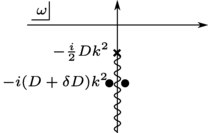
\begin{equation} \Sigma(\eta, \omega) = J^2\eta^2\left[1+\frac{1}{2}\sqrt{\eta^2-2i\omega}\right]. \label{eq:se-final-low} \end{equation}
The diffusion pole at $\omega=-i\eta^2$ becomes a pair
\begin{equation} \omega_\pm = -i(1+J^2)\eta^2 \pm |\eta|^3\frac{J^2}{2}\sqrt{1+2J^2} + O(\eta^4). \label{eq:poles} \end{equation}
Branch point $\omega=-i\eta^2/2$: min. $\omega(\eta_1)+\omega(\eta_2)$ when $\eta_{1,2}\to\eta/2$.
Analytic structure
Enhanced diffusion
\begin{equation} \omega = -i(1+J^2)\eta^2 \pm |\eta|^3\frac{J^2}{2}\sqrt{1+2J^2} + O(\eta^4). \end{equation}
$J$ enhances ordinary diffusion
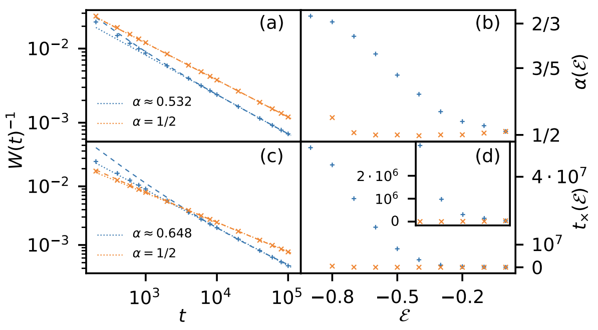
Find transient diffusion constant using $D(t) = -\frac{1}{2} \left. \partial_t\partial^2_\eta C^z(\eta;t) \right\vert_{\eta=0}$
\begin{align} D(t) = 1 + J^2 - J^2 e^{-4t}\left[I_0(4t)+I_1(4t)\right]\ \underset{t\to\infty}{\longrightarrow} 1 + J^2 - \frac{J^2}{\sqrt{2\pi t}} \end{align}
Numerics
Represent $Z_j(t)$ using MPO and evolve using TEBD (based on TeNPy)
$\chi = 400$, truncation error $\epsilon = 10^{−12}$, $\delta t = 10^{-2}$
Exact for $J=0$ ($\chi=2$)
Diffusion constant
- 100 spins
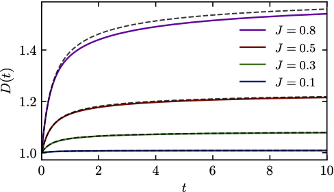
- Analytic calculation (dashed) upper bounds $D(t)$
Profile
\begin{equation} \omega = -i(1+J^2)\eta^2 \pm |\eta|^3\frac{J^2}{2}\sqrt{1+2J^2} + O(\eta^4). \end{equation}
- Assuming poles dominate profile saddle point analysis yields
\begin{align}\label{eq:saddlepointprofile} C(x;t) \propto \exp\left(-\frac{x^2}{2Dt}\right)\exp\left(-\frac{J^2 \sqrt{2J^2+1}}{2 D^3}\frac{|x|^3}{t^2}\right) \end{align}
- 2nd factor hints at $\ell\sim t^{2/3}$ for KPZ!
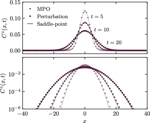
\begin{align} C(x;t) \propto \exp\left(-\frac{x^2}{2Dt}\right)\exp\left(-\frac{J^2 \sqrt{2J^2+1}}{2 D^3}\frac{|x|^3}{t^2}\right) \end{align}
Nonabelian hydrodynamics
- Glorioso et al. (2020): corrections to current
$$ J^a = -D\nabla s^a + \lambda \epsilon_{abc} s^b \nabla s^c $$
Implies $\sim \lambda^2/\sqrt{t}$ corrections to diffusion constant
Consistent with $D(t) \underset{t\to\infty}{\longrightarrow} 1 + J^2 - \frac{J^2}{\sqrt{2\pi t}}$
Higher orders?
- Recall 2nd order result
\begin{equation} \Sigma(\eta, \omega) = J^2\eta^2\left[1+\frac{1}{2}\sqrt{\eta^2-2i\omega}\right] \end{equation}
Branch point $\omega=-i\eta^2/2$: min. $\omega(\eta_1)+\omega(\eta_2)$ when $\eta_{1,2}\to\eta/2$.
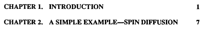
On kinematic grounds: at order $J^{2n}$ branch point at $\omega=-i\eta^2/n$: minimum $\omega(\eta_1)+\omega(\eta_2)+\cdots +\omega(\eta_n)$ for $\eta_{1,2,\ldots n}\to\eta/n$.
Diffuson cascade?
Contribution of $n$-diffusons is $\sim n! (k\ell_\text{th})^{nd}\exp\left(-\frac{Dk^2t}{n}\right)$
Optimal $n$ gives contribution $\sim \exp\left(-\alpha\sqrt{Dk^2|t|}\right)$
Would be interesting to see this in a microscopic model!
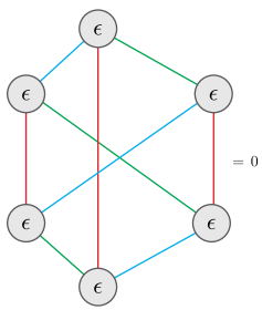
Penrose colouring
- Recall each vertex has $\epsilon_{abc}$. For planar graph this counts 3-colorings

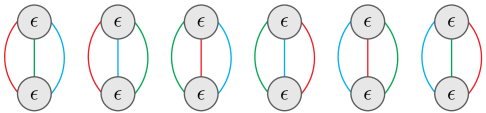
- Some graphs can’t be 3-colored
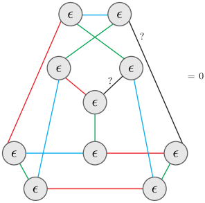
- Some non-planar graphs give zero