$$ \nonumber \newcommand{\bra}[1]{\langle{#1}\rvert} \newcommand{\ket}[1]{\lvert{#1}\rangle} \newcommand{\br}{\mathbf{r}} \newcommand{\bR}{\mathbf{R}} \newcommand{\bp}{\mathbf{p}} \newcommand{\bk}{\mathbf{k}} \newcommand{\bq}{\mathbf{q}} \newcommand{\bv}{\mathbf{v}} \newcommand{\bx}{\mathbf{x}} \newcommand{\bz}{\mathbf{z}} \DeclareMathOperator*{\E}{\mathbb{E}} $$
Superdiffusion in spin chains
Review: arXiv:2103.01976 Bulchandani, Gopalakrishnan, Ilievski
What?
Where?
How?
Diffusion
$$ \frac{\partial u}{\partial t} = D \frac{\partial^2 u}{\partial x^2} $$
- Fundamental solution of heat equation $$ u(x,t) = \frac{1}{\sqrt{4\pi Dt}}\exp\left[-\frac{(x-x_0)^2}{4Dt}\right] $$
- More generally have scaling solutions $u(x,t)\to \frac{1}{\sqrt{t}}f\left(\frac{x-x_0}{\sqrt{Dt}}\right)$
- Dynamical critical exponent $x\sim t^{1/z}$ with $z=2$
- $u(x,t)$ is conserved: $\int u(x,t) dx=\text{const.}$
Spin diffusion
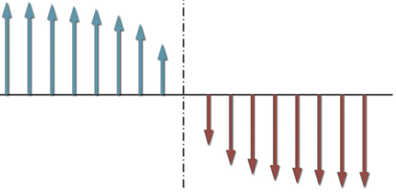
- Relaxation of inhomogeneity (e.g. domain wall)
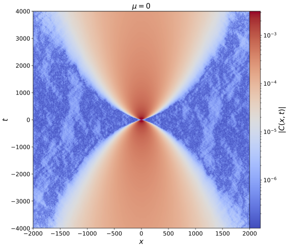
- Spin correlations $\langle Z(x,t)Z(x’,t’)\rangle$ as measured in neutron diffraction (say)
Models
Heisenberg spin-1/2 chain $$ H = \sum_j \left[X_j X_{j+1}+Y_j Y_{j+1}+ \Delta Z_j Z_{j+1}\right] $$
$\Delta=1$ is isotropic (XXX model). All 3 components conserved
$\Delta\neq 1$: Only $Z$ conserved
(Naive) expectation: $Z$ diffuses. In fact: something’s up at $\Delta=1$!
Numerics: steady state
- Žnidarič (2011) tDMRG with ends coupled to reservoirs with fixed chemical potentials

Steady state current $j\sim L^{-1/2}$. $j= D\frac{\partial s}{\partial x}$ suggests $D\sim L^{1/2}$
$\omega = Dk^2$ implies $\omega\sim k^{3/2}$ or $z=3/2$. Superdiffusion
Numerics: relaxation
- Ljubotina, Žnidarič, Prosen (2017) studied weak domain wall initial conditions
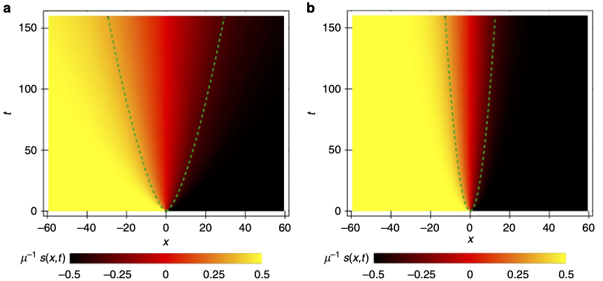
- Again, superdiffusion with $z=3/2$
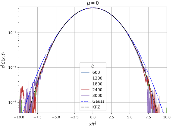
- In 2019, same authors improved accuracy and identified scaling behaviour with KPZ universality class (more later)
Numerics: classical
- Krajnik and Prosen (2020) introduced classical circuit
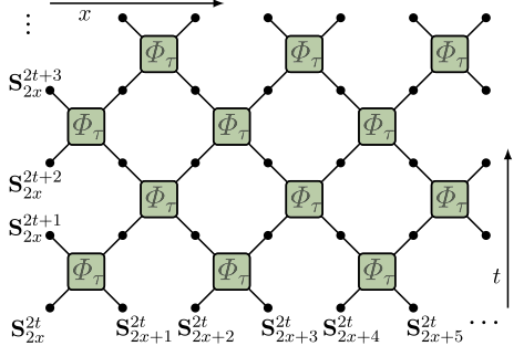
$$ \begin{align} \Phi_\tau(\mathbf{S}_1,\mathbf{S}_2) = \frac{1}{\sigma^2+\tau^2}&\left[\sigma^2 \mathbf{S}_1+\tau^2 \mathbf{S}_2 + \tau \mathbf{S}_1\times \mathbf{S}_2,\\ \sigma^2 \mathbf{S}_2+\tau^2 \mathbf{S}_1 + \tau \mathbf{S}_2\times \mathbf{S}_1\right] \end{align} $$
- $\sigma^2=\frac{1}{2}\left(1+\mathbf{S}_1\cdot \mathbf{S}_2\right)$
Features in common?
Non-abelian symmetry e.g. $SU(2)$ not $U(1)$
Integrability (extensive number of conservation laws)
Experiment
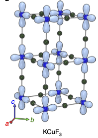
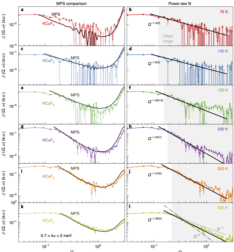
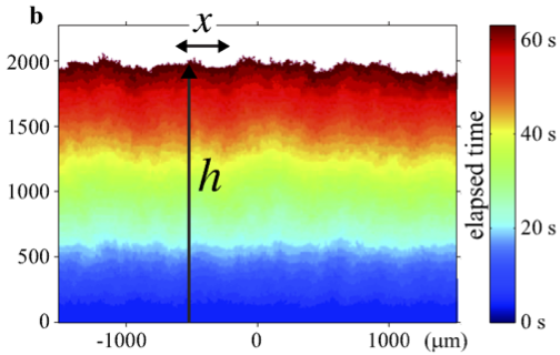
- Scheie et al observe KPZ scaling in 1D Heisenberg antiferromagnet KCuF3 with neutron scattering
KPZ equation
$$ \partial_t h = \partial_x^2 h + \frac{\lambda}{2}(\partial_x h)^2 + \overbrace{\xi(x,t)}^{\text{noise}} $$
Origin of $z=3/2$
KPZ is related to Burgers equation via $v=-\partial_x h$ (set $\lambda=1$) $$ \partial_t v + v\partial_x v = \partial_x^2 h + \partial_x\xi(x,t) $$
Scale $x\to \lambda x$, $t\to \lambda^z t$
Preserves Galilean invariance: $\partial_t v+v\partial_x v$ preserved
Steady state $v$ is white noise ($h$ is Brownian): $v\to \lambda^{-1/2}v$
Must have $z=1+\frac{1}{2}=\frac{3}{2}$ (Forster, Nelson, and Stephen (1977))
Much recent progress on scaling functions in 1+1 dimensions
Why KPZ?
Bulchandani (2020) suggests following (classical) picture
Landau–Lifshitz equation for magnetization density $\mathbf{s}(x,t)$ $$ \partial_t\mathbf{s} = \mathbf{s}\times \partial_x^2\mathbf{s} $$
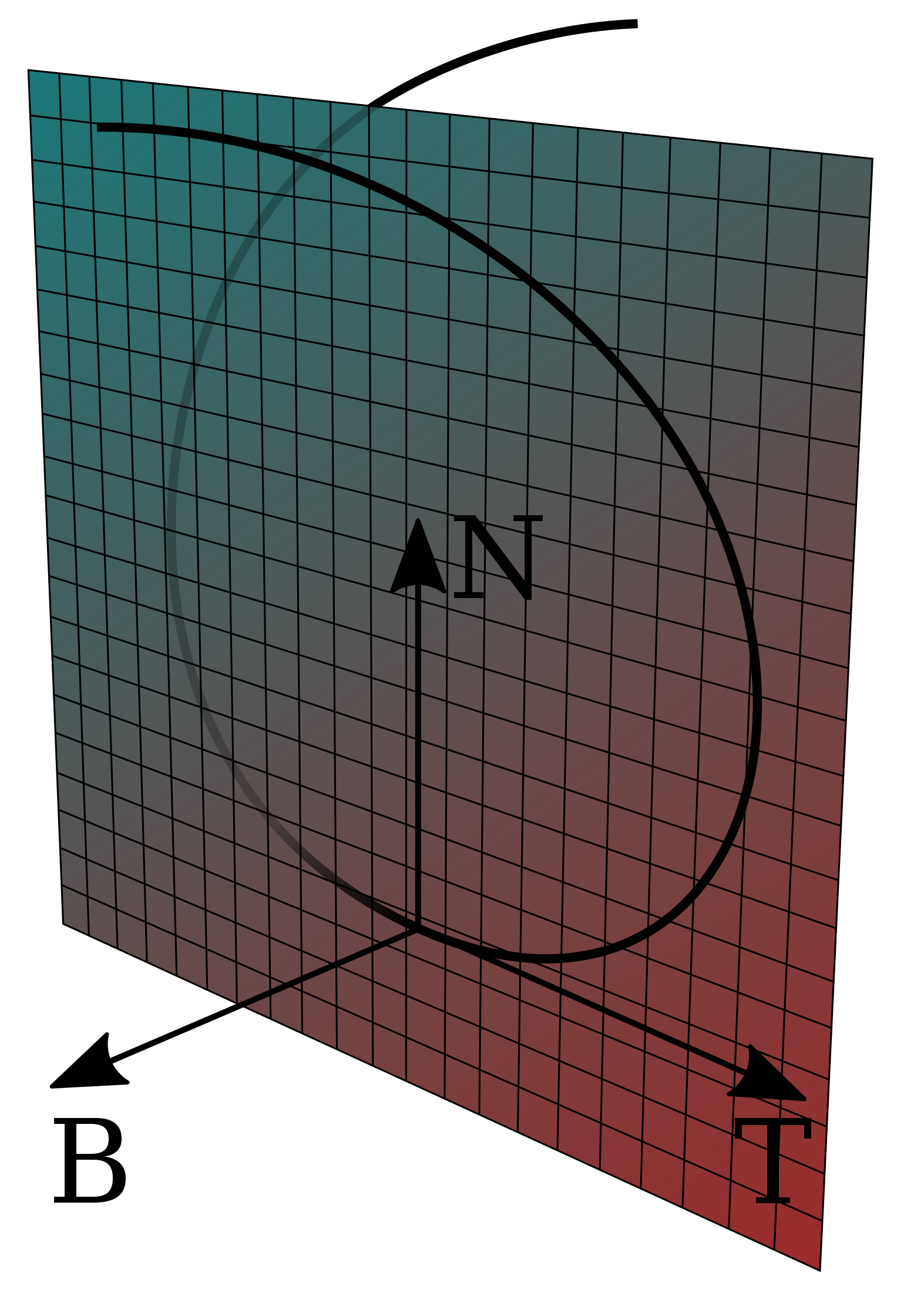
Regard $\mathbf{s}(x)=\mathbf{T}(x)$ as tangent vector of space curve, with $x$ as arc length
- With $\mathcal{E}\equiv \kappa^2/2$ LLE takes form (dropping higher derivative terms)
$$ \begin{align} \partial_t \mathcal{E} +2\partial_x\left(\mathcal{E}\tau\right)&=0\\ \partial_t \tau +\partial_x\left(\tau^2-\mathcal{E}\right)&=0 \end{align} $$
Linear instability!
If we can set $\mathcal{E}=0$ at long scales and coarse graining introduces noise and damping, then
$$ \partial_t \tau +\partial_x\left(\tau^2-D\partial_x\tau+\xi(x,t\right)=0 $$
- Noisy Burgers, hence KPZ
What’s missing?
- A straight-through calculation starting from a microscopic model
A model with a small parameter
Fluctuating exchange interaction $$ d\ket{\psi} = \sum_j \left[-i(J dt + dW_j)P_{j,j+1}-\frac{1}{2}dt\right]\ket{\psi}. $$ (last term is there to ensure that the norm is preserved)
Heisenberg equation of motion $$ d\mathcal{O} = \sum_j i\left[\left(J dt + dW_j\right)P_{j,j+1},\mathcal{O}\right]+dt\left(P_{j,j+1}\mathcal{O}P_{j,j+1}-\mathcal{O}\right). $$
- $\bar{\mathcal{O}}\equiv\E \mathcal{O}$ obeys Lindblad equation
$$ \begin{equation} \frac{d\bar{\mathcal{O}}}{dt} = \sum_j iJ \left[P_{j,j+1},\bar{\mathcal{O}}\right]+\left(P_{j,j+1}\bar{\mathcal{O}}P_{j,j+1}-\bar{\mathcal{O}}\right) \end{equation} $$
- Expand in components
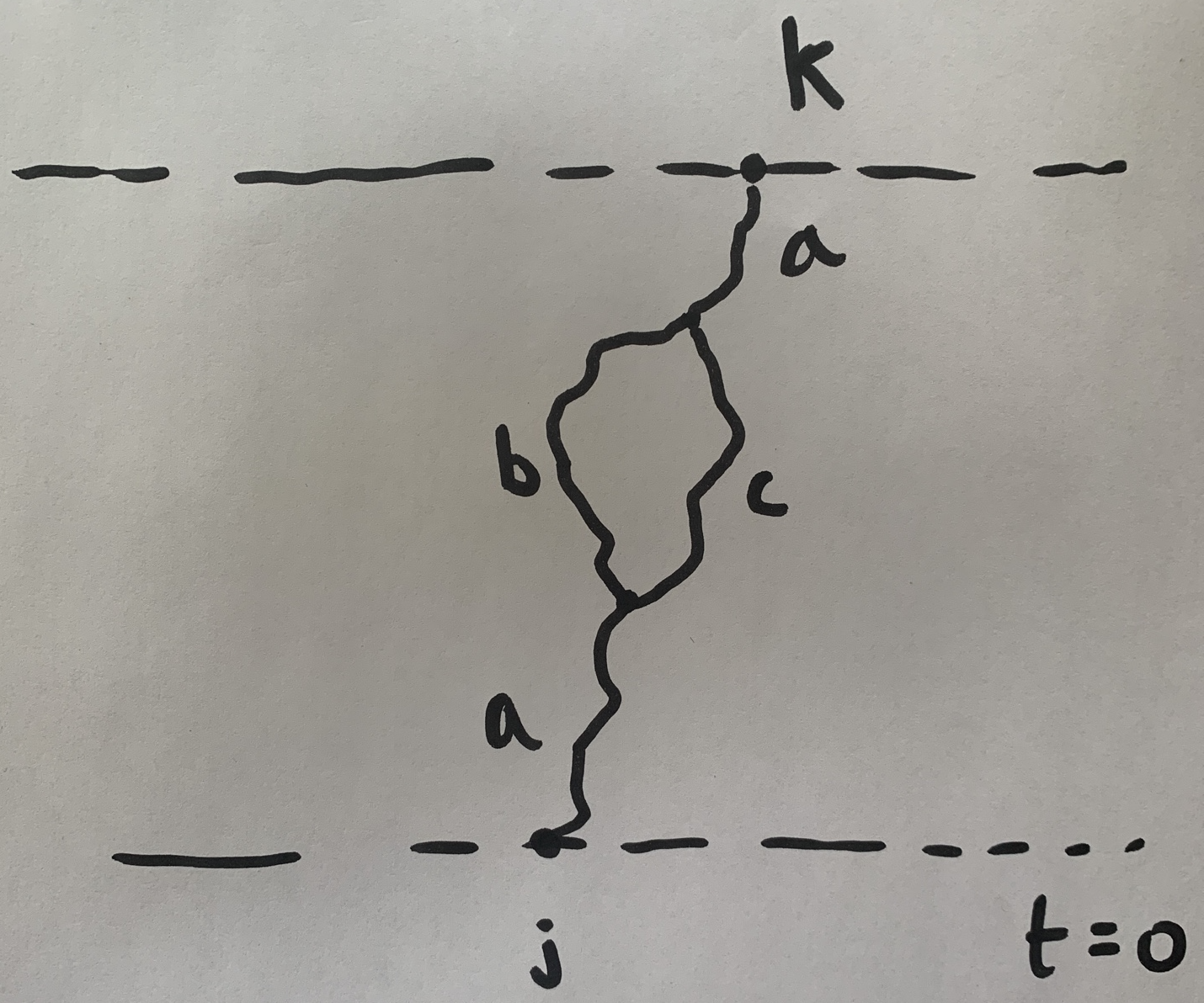
$$ \mathcal{O}= \sum_{\mu_{1:N}=\{0,1,2,3\}^N} \mathcal{C}^a_{\mu_{1:N}}(t) \sigma_1^{\mu_1}\otimes\cdots \sigma_N^{\mu_N}, $$
$$ \partial_t \mathcal{C}_{\mu_{1:N}} = \sum_j \left[J\sum_{\alpha\beta} \epsilon_{\alpha\beta \mu_j \mu_{j+1}} \mathcal{C}_{\mu_1\cdots \alpha\beta \cdots \mu_N} + \mathcal{C}_{\mu_1\cdots \mu_{j+1}\mu_j \cdots \mu_N} - \mathcal{C}_{\mu_1\cdots \mu_{j}\mu_{j+1} \cdots \mu_N}\right] $$
$$ \partial_t \mathcal{C}_{\mu_{1:N}} = \sum_j \left[J\sum_{\alpha\beta} \epsilon_{\alpha\beta \mu_j \mu_{j+1}} \mathcal{C}_{\mu_1\cdots \alpha\beta \cdots \mu_N} + \mathcal{C}_{\mu_1\cdots \mu_{j+1}\mu_j \cdots \mu_N} - \mathcal{C}_{\mu_1\cdots \mu_{j}\mu_{j+1} \cdots \mu_N}\right] $$
$J=0$ describes operator diffusion
$J\neq 0$ describes splitting and merging e.g. $Z_j\leftrightarrow X_jY_{j+1}$